Download
1 / 13
130 likes | 152 Views
Learn about count data models, examples like doctor visits, Poisson distribution, estimation techniques, and other distributions including negative binomial. Explore the impact of overdispersion, probability calculations, and interpretation of results in regression analysis.

E N D
Jacek Wallusch_________________________________Introduction to Econometrics Lecture 4: Count Data Models
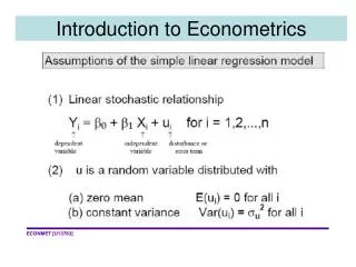
Count Data____________________________________________________________________________________________ definitions Count 1.to name numbers in regular order; 2. to have a specified value [a touchdown counts for six points]*; Integer 1. anything complete in itself; entity; 2. any positice or negative whole number or zero; ItE: 4 Webster’s New World College Dictionary * That’s Webster as well!!!
Count Data____________________________________________________________________________________________ Example Doctor Visits:number of doctor visits per one respondent within a specified period of time explanatory variables: socioeconomic – gender, age, squared age, income health insurance status indicators – insured, not insured recent health status measure – number of illnesses in past 2 weeks, number of days of reduced activity long-term health status measure – health questionnaire score ItE: 4 Example: Cameron and Trivedi 1998
Count Data____________________________________________________________________________________________ Example Doctor Visits:see cont_docvisits.xls exlaining variable:avg. = 6.823 std.dev. = 7.395 skew = 4.176 kurt = 46.744 ItE: 4 Example: Katchova 2013
Count Data____________________________________________________________________________________________ Examples Other Topics: research and development: patents granted, domestic patents, foreign patents etc. sales: number of items sold quality control: number of defective items produced Important note: time structure and/or cross-section ItE: 4
Count Data____________________________________________________________________________________________ Background Poisson distribution and rare events Poisson density: expected value and variance: Warning: equidispersion property is often violated in practice, i.e. ItE: 4 m – intensity (rate) coefficient, t – exposure (length of time during which the events are recorded)
Estimation____________________________________________________________________________________________Estimation____________________________________________________________________________________________ coefficients Poisson distribution and rare events The model: left-hand variable y: number of occurences of the event of interest (e.g. doctor visits) mean coefficient: ItE: 4 b – coefficient vector, x – vector of linearly independent regressors
Probability____________________________________________________________________________________________Probability____________________________________________________________________________________________ Poisson model Poisson distribution and estimatedprobabilities Using the estimated mean to calculate probabilities: condition Conditional probability that the left hand variable = y ItE: 4 b – coefficient vector, x – vector of linearly independent regressors
Other Distributions____________________________________________________________________________________________ negative binomial Important limitation: Overdispersion Solution: negative binomial model mean coefficient: variance: ItE: 4 r – number of trials at wich success occurs, p – probability of success
Distributions____________________________________________________________________________________________Distributions____________________________________________________________________________________________ examples Randomly generated distributions descriptive statistics: ItE: 4
Results____________________________________________________________________________________________Results____________________________________________________________________________________________ Interpretation Marginal Effects Exponential conditional mean: differentiation: Procedures: ItE: 4 (1) average response after aggregating over all individuals vs. (2) response for the individual with average characteristics
Methods of Estimatios____________________________________________________________________________________________ Overdispersion GRETL Test for overdispersion: null hypothesis: no overdispersion interpretation: rejection of the null suggests the need for different distribution ItE: 4
Methods of Estimatios____________________________________________________________________________________________ Overdispersion GRETL NEG BIN 2: a-coefficient: measure of heterogeneity between individuals NEG BIN 1: conditional variance: scalar multiple (g) of conditional mean ItE: 4