Download
1 / 50
920 likes | 2.48k Views
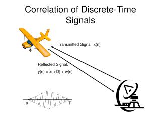
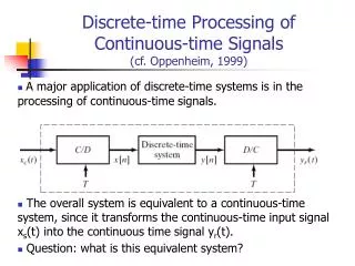
Discrete-time Processing of Continuous-time Signals (cf. Oppenheim, 1999). A major application of discrete-time systems is in the processing of continuous-time signals.

E N D
Discrete-time Processing of Continuous-time Signals(cf. Oppenheim, 1999) • A major application of discrete-time systems is in the processing of continuous-time signals. • The overall system is equivalent to a continuous-time system, since it transforms the continuous-time input signal xs(t) into the continuous time signal yr(t). • Question: what is this equivalent system?
Ideal reconstruction filter The ideal reconstruction filter is a continuous-time filter, with the frequency response being Hr(j) and impulse response hr(t). From now on, we use to represent the transform domain of continuous Fourier transform.
continuous F. T. Continuous to discrete (C/D) converter where s = 2/T Time domain multiplication
where s = 2/T C/D converter Frequency domain convolution We have • Hence, the continuous Fourier transforms of xs(t) consists of periodically repeated copies of the Fourier transform of xc(t). • Review of Nyquist sampling theorem: • Aliasing effect: If s > 2N, the copies of Xc(j) overlap, where N is the highest nonzero frequency component of Xc(j). N is referred to as the Nyquist frequency.
Ideal C/D converter • In the above, we characterize the relationship of xs(t) and xc(t) in the continuous F.T. domain. • From another point of view, Xs(j) can be represented as the linear combination of a serious of complex exponentials: • If x(nT) x[n], its DTFT is
Input-output relationship of C/D converter • Combining these properties, we have the relationship between the continuous F.T. and DTFT of the sampled signal: where : represent continuous F.T. : represent DTFT • Thus, we have the input-output relationship of C/D converter
Combine C/D, discrete-time system, and D/C • Consider again the discrete-time processing of continuous signals • Let H(ejw) be the frequency response of the discrete-time system in the above diagram. Since Y(ejw) = H(ejw)X(ejw)
D/C converter revisited • An ideal low-pass filter Hr(j) that has a cut-off frequency c= s/2 = /T and gain T is used for reconstructing the continuous signal. • Frequency domain of D/C converter: (Hr(j) is its frequency response) • Remember that the corresponding impulse response is a sinc function, and the reconstructed signal is
Input-output Relationship for Discrete-time processing of continuous-time signals Assumption: If Xc(j) is band limited with Xc(j) = 0 for ||>/T, then and hence
Effective Frequency Response for Discrete-time processing of continuous-time signals So, if Xc(j) is band limited with Xc(j) = 0 for ||>/T, we have the following effective response for the entire system:
Effective Frequency Response • It is important to emphasize that the LTI behavior of the system depends on two factors: • First, the discrete-time system is LTI. • Second, the input signal is band-limited, and the sampling rate is high enough so that any aliased components are removed.
Discrete-time processing of continuous-time signals • If we are given a desired continuous-time system with band-limited frequency response Hc(j), and we want to implement it by discrete-time processing, • We can choose appropriate T and discrete-time filter satisfying H(ejw) = Hc(jw/T) to synthesize the continuous response Hc(j).
Time-domain behavior of discrete-time processing of continuous-time signals • In time domain • Since H(ejw) = Hc(jw/T) |w| < • In addition, Hc(j) = 0, ||>/T (band limited) • We have the impulse invariance property, h[n]=Thc(nT), i.e., the impulse response of the discrete-time system is a scaled, sampled version of the continuous inpulse response hc(t). Remark: It is because that if and thus since band limited.
Continuous-time processing of discrete-time signals • On the other hand, we can also consider to process discrete-time signal with continuous-time filters. • Cascading D/C, continuous-time system, and C/D. • From the definition of the ideal D/C converter, Xc(j) and therefore also Yc(j), will necessarily be zero for ||>/T.
Continuous-time processing of discrete-time signals • Hence, we have the effective system of the continuous-time processing of discrete-time signals to be
Changing the Sampling rate using discrete-time processing • downsampling; sampling rate compressor;
Frequency domain of downsampling • Since this is a ‘re-sampling’ process. Remember that, from continuous-time sampling of x[n]=xc(nT), we have • Similarly, for the down-sampled signal xd[m]=xc(mT’), (where T’ = MT), we have
Frequency domain of downsampling • We are interested in the relation between X(ejw) and Xd(ejw). Let’s represent r as r = i + kM, where 0 i M1, (i.e., r i (mod M)). Then
Frequency domain of downsampling • Therefore, the downsampling can be treated as a ‘re-sampling’ process. It s frequency domain relationship is similar to that of the D/C converter as: • This is equivalent to compositing M copies of the of X(ejw), frequency scaled by M and shifted by inter multiples of 2. • The aliasing can be avoided by ensuring that X(ejw) is bandlimited as
Example of downsampling in the Frequency domain (without aliasing) Sampling with a sufficiently large rate which avoids aliasing
Example of downsampling in the Frequency domain (without aliasing) Downsampling by 2 (M=2)
Downsampling with prefiltering to avoid aliasing (decimation) • From the above, the DTFT of the down-sampled signal is the superposition of M shifted/scaled versions of the DTFT of the original signal. • To avoid aliasing, we need wN</M, where wN is the highest frequency of the discrete-time signal x[n]. • Hence, downsampling is usually accompanied with a pre-low-pass filtering, and a low-pass filter followed by down-sampling is usually called a decimator, and termed the process as decimation.
Up-sampling • Upsampling; sampling rate expander. or equivalently, In frequency domain: :
Example of up-sampling Upsampling in the frequency domain
Up-sampling with post low-pass filtering • Similar to the case of D/C converter, upsampoling is usually companied with a post low-pass filter with cutoff frequency /L and gain L, to reconstruct the sequence. • A low-pass filter followed by up-sampling is called an interpolator, and the whole process is called interpolation.
Example of up-sampling followed by low-pass filtering Applying low-pass filtering
Interpolation • Similar to the ideal D/C converter, • If we choose an ideal lowpass filter with cutoff frequency /L and gain L, its impulse response is • Hence Its an interpolation of the discrete sequence x[k]
Sampling rate conversion by a non-integer rational factor • By combining the decimation and interpolation, we can change the sampling rate of a sequence. • Changing the sampling rate by a non-integer factor T’ = TM/L. • Eg., L=100 and M=101, then T’ = 1.01T.
Changing the Sampling rate using discrete-time processing • Since the interpolation and decimation filters are in cascade, they can be combined as shown above.
Digital Processing of Analog Signals • Pre-filtering to avoid aliasing • It is generally desirable to minimize the sampling rate. • Eg., in processing speech signals, where often only the low-frequency band up to about 3-4k Hz is required, even though the speech signal may have significant frequency content in the 4k to 20k Hz range. • Also, even if the signal is naturally bandlimited, wideband additive noise may fll in the higher frequency range, and as a result of sampling. These noise components would be aliased into the low frequency band.
Over-sampled A/D conversion • The anti-aliasing filter is an analog filter. However, in applications involving powerful, but inexpensive, digital processors, these continuous-time filters may account for a major part of the cost of a system. • Instead, we first apply a very simple anti-aliasing filter that has a gradual cutoff (instead of a sharp cutoff) with significant attenuation at MN. Next, implement the C/D conversion at the sampling rate higher than 2MN. After that, sampling rate reduction by a factor of M that includes sharp anti-aliasing filtering is implemented in the discrete-time domain.
Using over-sampled A/D conversion to simplify a continuous-time anti-aliasing filter
Quantizer (Quantization) • The real-valued signal has to be stored as a code for digital processing. This step is called quantization. • The quantizer is a nonlinear system. • Typically, we apply two’s complement code for representation.
Quantizer (Quantization) • In general, if we have a (B+1)-bit binary two’s complement fraction of the form: then its value is • The step size of the quantizer is where Xm is the full scale level of the A/D converter. • The numerical relationship beween the code words and the quantizer samples is
Analysis of quantization errors • Quantization error • In general, for a (B+1)-bit quantizer with step size , the quantization error satisfies that when • If x[n] is outside this range, then the quantization error is larger in magnitude than /2, and such samples are saided to be clipped.
Analysis of quantization errors • Analyzing the quantization by introducing an error source and linearizing the system: • The model is equivalent to quantizer if we know e[n].
Assumptions about e[n] • e[n] is a sample sequence of a stationary random process. • e[n] is uncorrelated with the sequence x[n]. • The random variables of the error process e[n] are uncorrelated; i.e., the error is a white-noise process. • The probability distribution of the error process is uniform over the range of quantization error (i.e., without being clipped). • The assumptions would not be justified. However, when the signal is a complicated signal (such as speech or music), the assumptions are more realistic. • Experiments have shown that, as the signal becomes more complicated, the measured correlation between the signal and the quantization error decreases, and the error also becomes uncorrelated.
Example of quantization error original signal 3-bit quantization result 3-bit quantization error
Example of quantization error 8-bit quantization error • In a heuristic sense, the assumptions of the statistical model appear to be valid if the signal is sufficiently complex and the quantization steps are sufficiently small, so that the amplitude of the signal is likely to traverse many quantization steps from sample to sample.
Quantization error analysis • e[n] is a white noise sequence. The probability density function of e[n] is
Quantization error analysis • The mean value of e[n] is zero, and its variance is • Since For a (B+1)-bit quantizer with full-scale value Xm, the noise variance, or power, is
Quantization error analysis • A common measure of the amount of degradation of a signal by additive noise is the signal-to-noise ratio (SNR), defined as the ratio of signal variance (power) to noise variance. Expressed in decibels (dB), the SNR of a (B+1)-bit quantizer is • Hence, the SNR increases approximately 6dB for each bit added to the world length of the quantized samples.
Quantization error analysis • The equation can be further simplified for analysis. For example, if the signal amplitude has a Gaussian distribution, only 0.064 percent of the samples would have an amplitude greater than 4x. • Thus to avoid clipping the peaks of the signal (as is assumed in our statistical model), we might set the gain of filters and amplifiers preceding the A/D converter so that x = Xm/4. Using this value of x gives • For example, obtaining a SNR about 90-96 dB in high-quality music recording and playback requires 16-bit quantization. • But it should be remembered that such performance is obtained only if the input signal is carefully matched to the full-scale of the A/D converter.