Download

1 / 105
1.24k likes | 1.94k Views
1. Time Domain Representation of Signals and Systems 1.1 Discrete-Time Signals 1.2 Operations on Sequences 1.3 Classification of Sequences 1.4 Some Basic Sequences 1.5 The Sampling Process 1.6 Discrete-Time Systems

E N D
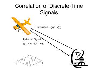
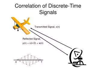
1. Time Domain Representation of Signals and Systems 1.1 Discrete-Time Signals 1.2 Operations on Sequences 1.3 Classification of Sequences 1.4 Some Basic Sequences 1.5 The Sampling Process 1.6 Discrete-Time Systems 1.7 Classification of Discrete-Time Systems 1.8 Time-Domain Characterization of LTI Systems 1.9 Correlation
1.1 Discrete-Time Signals • There are basically two types of discrete time signals: • Sampled-data signalsin which samples are continuous-valued • digital signalsin which samples are discrete-valued • Digital signals are obtained by quantizing the sample values either by rounding or truncation
Discrete-Time Signals • Signals are represented as sequences of numbers, called samples • A sample value of a typical signal or sequence is denoted as x[n] with n being an integer in the range • x[n] is defined only for integer values of n and is undefined for non-integer values of n • Discrete-time signal represented by {x[n]}
Discrete-Time Signals • Discrete-time signal may also be written as a sequence of numbers inside braces: x[n]={…,-0.2, 2.2,1.1,0.2,-0.7,2.9,…} • In the above, x[-1]=-0.2, x[0]=2.2 x[1]=1.1 etc. • The arrow is placed under the sample at time index n = 0
Discrete-Time Signals • The graphical representation of a discrete time signal with real-valued samples is as shown below:
Discrete-Time Signals • In some applications, a discrete-time sequence {x[n]} may be generated by periodically sampling a continuous-time signal xa(t) at uniform time intervals
Discrete-Time Signals • Here, n-th sample is given by: x[n]= xa(t)|t=nT= xa(nT), n=…,-2,-1,0,1,… • The spacing T between two consecutive samples is called the sampling intervalor sampling period • Reciprocal of sampling interval T, denoted as FT is called sampling frequency: FT=1/T
Discrete-Time Signals • Whether or not the sequence {x[n]} has been obtained by sampling, the quantity, x[n] is called the n-th sampleof the sequence • {x[n]} is a real sequence, if the n-th sample x[n] is real for all values of n • Otherwise, {x[n]} is a complex sequence
Discrete-Time Signals • A complex sequence {x[n]} can be written as {x[n]}={xre[n]+jxim[n]} where xre[n] and xim[n] are the real and imaginary parts of x[n] • The complex conjugate sequence of {x[n]} is given by {x*[n]}={xre[n]- jxim[n]} • Often the braces are ignored to denote a sequence if there is no ambiguity
Discrete-Time Signals • A discrete-time signal may be a finite length or an infinite-length sequence • Finite-length (also called finite-durationor finite-extent) sequence is defined only for a finite time interval: where: with • Lengthor durationof the above finite length sequence is N=N2-N1+1
Discrete-Time Signals • Examples: x[n]= n2, is a finite-length sequence of length 8 y[n]=cos(0.4n) is an infinite-length sequence
Discrete-Time Signals • A length-N sequence is often referred to as an N-point sequence • The length of a finite-length sequence can be increased by zero-padding, ie: by appendingit with zeros
Discrete-Time Signals • Example: is a finite-length sequence of length-12 obtained by zero-padding the sequence with 4 zero-valued samples
Discrete-Time Signals • A right-sided sequence x[n] has zero valued samples for • Ifa right-sided sequence is called a causal sequence
Discrete-Time Signals • A left-sided sequence x[n] has zero-valued samples for • If a left-sided sequence is called a anti-causal sequence
1.2 Operations on Sequences • A single-input, single-output discrete-time system operates on a sequence, called the input sequence, according some prescribed rules and develops another sequence, called the output sequence, with more desirable properties
Operations on Sequences • For example, the input may be a signal corrupted with additive noise • Discrete-time system is designed to generate an output by removing the noise component from the input • In most cases, the operation defining a particular discrete-time system is composed of some basic operationsthat we describe next:
Basic Operations • Product(modulation)operation: y[n]=x[n].w[n] Modulator: • An application is in forming a finite-length sequence from an infinite-length sequence by multiplying with a window sequence • This process is usually called windowing
Basic Operations • Additionoperation: y[n]=x[n]+w[n] Adder: • Multiplicationoperation: y[n] = A.x[n] • Multiplier:
Basic Operations • Time-shiftingoperation: y[n] = x[n − N] , where N is an integer • If N > 0, it is delayingoperation e.g. unit delay: y[n] = x[n −1] • If N < 0, it is an advanceoperation, e.g. unit advance: y[n] = x[n +1]
Basic Operations • Time-reversaloperation: y[n] = x[−n] • Branchingoperation: Used to provide multiple copies of a sequence
Basic Operations • Example: Consider the two following sequences of length 5 defined for 0 ≤ n ≤ 4: {a[n]}={3 4 6 − 90} {b[n]}={2 −1 4 5 −3} • New sequences generated from the above two sequences by applying the basic operations are as follows:
Basic Operations {c[n]}= {a[n]⋅b[n]}= {6 − 4 24 − 450} {d[n]}= {a[n]+ b[n]}= {5 3 10 − 4 −3} {e[n]}={4.5 6 9 13.50} • As pointed out by the above examples, operations on two or more sequences can be carried out if all sequences involved are of same length and defined for the same range of the time index n
Basic Operations • However if the sequences are not of same length, in some situations, this problem can be circumvented by appending zero-valued samples to the sequence(s) of smaller lengths to make all sequences have the same range of the time index • Example: Consider the sequence of length 3 • defined for 0 ≤ n ≤ 2 :{f [n]}= {− 2 1 −3}
Basic Operations • We cannot add the length-3 sequence to the length-5 sequence {a[n]} defined earlier • We therefore first append {f [n]} with 2 zero-valued samples resulting in a length-5 sequence {fe[n]}= {− 2 1 − 3 0 0} • Then {g[n]} ={a[n]}+{fe[n]} ={1 5 3 − 9 0}
Combinations of Basic Operations • Example: y[n] =α1x[n]+α 2x[n −1]+α3x[n − 2]+α4x[n − 3]
1.3 Classification of Sequences Based on Symmetry • Conjugate-symmetric sequence: x[n] = x*[−n] • If x[n] is real, then it is an even sequence An Even Sequence
Classification of Sequences Based on Symmetry • Conjugate-antisymmetric sequence: x[n] = −x*[−n] • If x[n] is real, then it is an odd sequence An Odd Sequence
Classification of Sequence Based on Symmetry • It follows from the definition that for a conjugate-symmetric sequence {x[n]}, x[0] must be a real number • Likewise, it follows from the definition that for a conjugate-antisymmetric sequence {y[n]}, y[0] must be an imaginary number • From the above, it also follows that for an odd sequence {w[n]}, w[0] = 0
Classification of Sequences Based on Symmetry • Any complex sequence can be expressed as a sum of its conjugate-symmetric part and its conjugate-antisymmetric part, if the parent sequence is of odd length defined for a symmetric interval,−M ≤ 0 ≤ M: x[n] = xcs[n]+xca[n] where xcs[n]=1/2(x[n]+x*[-n]) xca[n]=1/2(x[n]-x*[-n])
Classification of Sequences Based on Symmetry • Example: Consider the complex length-7 sequence defined for − 3 ≤ n ≤ 3: {g[n]} = {0, 1+ j4, −2+ j3, 4− j2, −5− j6, −j2,3} • Its conjugate sequence is then given by: {g*[n]} = {0, 1− j4, −2− j3, 4+ j2, −5+ j6, j2,3} • The time-reversed version of the above is: {g*[−n]} = {3, j2, −5+ j6, 4+ j2, −2− j3,1−j4,0}
Classification of Sequences Based on Symmetry • Therefore {gcs[n]}=1/2{g[n]+ g *[−n]} ={1.5, 0.5+ j3, −3.5+ j4.5, 4, −3.5− j4.5, 0.5− j3, 1.5} • Likewise {gca[n]}=1/2 {g[n]− g *[−n]} ={−1.5, 0.5+ j, 1.5− j1.5, − j2, −1.5− j1.5, −0.5− j, 1.5} • It can be easily verified that gcs[n]= gcs*[-n]= and gca[n] = − gca*[-n]
Classification of Sequences: Periodic and Aperiodic Signals • A sequence x[n] satisfying: x[n]=x[n+kN] is called a periodic sequencewith a periodN where N is a positive integer and k is any integer • Smallest value of N satisfying x[n]=x[n+kN] is called the fundamental period
Classification of Sequences: Periodic and Aperiodic Signals • Example: Periodic sequence with period N=7 • A sequence not satisfying the periodicity • condition is called an aperiodic sequence
Classification of Sequences: Energy and Power Signals • The total energyof a sequence x[n] is defined by: • An infinite length sequence with finite sample values may or may not have finite energy • A finite length sequence with finite sample values has finite energy
Classification of Sequences: Energy and Power Signals • The average powerof an aperiodic sequence is defined by: • Now, we define the energyof a sequence x[n] over a finite interval − K ≤ n ≤ K as:
Classification of Sequences: Energy and Power Signals • Then, the average poweris: • The average powerof a periodic sequence x[n] with a period N is given by: • The average power of an infinite-length sequence may be finite or infinite
Classification of Sequences: Energy and Power Signals • Example: Consider the causal sequence defined by: • x[n] has infinite energy and its average power • is given by:
Classification of Sequences: Energy and Power Signals • An infinite energy signal with finite average power is called a power signal • Example: A periodic sequence which has a finite average power but infinite energy • A finite energy signal with zero average power is called an energy signal • Example: A finite-length sequence which has finite energy but zero average power:
Classification of Sequences: Other Types of Classifications • A sequence x[n] is said to be boundedif each of its samples is of magnitude less than or equal to a finite positive number Bx, i.e., • Example: The sequence x[n]=cos(0.3πn) is a bounded sequence as: |x[n]| = |cos0.3πn| ≤1
Classification of Sequences: Other Types of Classifications • A sequence x[n] is said to be absolutely summableif: Example: is an absolutely summable sequence as:
1.4 Some Basic Sequences • Unit sample sequence: • Unit step sequence:
Some Basic Sequences • Unit impulse and unit step sequence shifted by k samples: • Relations between the unit sample and the step sequence:
Some Basic Sequences • Real sinusoidal sequence: x[n] = Asin(ωon + φ) where A is the amplitude, ωo is the angularfrequency, and is the phaseof x[n] • Example:
Some Basic Sequences • Exponential sequence: x[n] = Aαn, − ∞ < n < ∞ where A and α are real or complex numbers • If we write: then we can express: where:
Some Basic Sequences • x [n] of a complex exponential sequence are real sinusoidal sequences with constant (σo= 0), growing (σo > 0) or decaying (σo < 0) amplitudes for n > 0 • Example: x[n] exp(-1/12+jπ/6)n
Some Basic Sequences • Real exponential sequence: x[n] =Aαn, −∞ < n < ∞ where A and α are real numbers. Example:
Some Basic Sequences • The sinusoidal sequence Asin(ωon + φ) and the complex exponential sequence Bexp( jωon) are periodic sequences of period N as long as ωoN = 2πr where N and r are positive integers • The smallest possible value of N satisfying ωoN = 2πr is the fundamental period
Some Basic Sequences • If 2π/ωois a noninteger rational number, then the period will be a multiple of 2π/ωo • Otherwise, the sequence is aperiodic • Example: x[n] = sin( 3n + φ) is aperiodic even though it has a sinusoidal envelope
Some Basic Sequences • Example: Period of Acos(ωon + φ) ωo= 0.1π Period N=2πr/0.1π=20 for r=1