Operations on Continuous-Time Signals
270 likes | 712 Views
Operations on Continuous-Time Signals. David W. Graham EE 327. Continuous-Time Signals. Continuous-Time Signals Time is a continuous variable The signal itself need not be continuous We will look at several common continuous-time signals and also operations that may be performed on them.

Operations on Continuous-Time Signals
E N D
Presentation Transcript
Operations on Continuous-Time Signals David W. Graham EE 327
Continuous-Time Signals • Continuous-Time Signals • Time is a continuous variable • The signal itself need not be continuous • We will look at several common continuous-time signals and also operations that may be performed on them
Unit Step Function u(t) • Used to characterize systems • We will use u(t) to illustrate the properties of continuous-time signals
Operations of CT Signals • Time Reversal y(t) = x(-t) • Time Shifting y(t) = x(t-td) • Amplitude Scaling y(t) = Bx(t) • Addition y(t) = x1(t) + x2(t) • Multiplication y(t) = x1(t)x2(t) • Time Scaling y(t) = x(at)
Solution: Find y(t) = u(-t) Let “a” be the argument of the step function u(a) Let a = -t, and plug in this value of “a” 1. Time Reversal • Flips the signal about the y axis • y(t) = x(-t) ex. Let x(t) = u(t), and perform time reversal
2. Time Shifting / Delay • y(t) = x(t – td) • Shifts the signal left or right • Shifts the origin of the signal to td • Rule Set (t – td) = 0 (set the argument equal to zero) Then move the origin of x(t) to td • Effectively, y(t) equals what x(t) was td seconds ago
Method 1 Let “a” be the argument of “u” 2. Time Shifting / Delay ex. Sketch y(t) = u(t – 2) Method 2 (by inspection) Simply shift the origin to td = 2
3. Amplitude Scaling • Multiply the entire signal by a constant value • y(t) = Bx(t) ex. Sketch y(t) = 5u(t)
4. Addition of Signals • Point-by-point addition of multiple signals • Move from left to right (or vice versa), and add the value of each signal together to achieve the final signal • y(t) = x1(t) + x2(t) • Graphical solution • Plot each individual portion of the signal (break into parts) • Add the signals point by point
4. Addition of Signals ex. Sketch y(t) = u(t) – u(t – 2) • First, plot each of the portions of this signal separately • x1(t) = u(t) Simply a step signal • x2(t) = –u(t-2) Delayed step signal, multiplied by -1 Then, move from one side to the other, and add their instantaneous values
5. Multiplication of Signals • Point-by-point multiplication of the values of each signal • y(t) = x1(t)x2(t) • Graphical solution • Plot each individual portion of the signal (break into parts) • Multiply the signals point by point
5. Multiplication of Signals ex. Sketch y(t) = u(t)∙u(t – 2) • First, plot each of the portions of this signal separately • x1(t) = u(t) Simply a step signal • x2(t) = u(t-2) Delayed step signal Then, move from one side to the other, and multiply instantaneous values
6. Time Scaling • Speed up or slow down a signal • Multiply the time in the argument by a constant • y(t) = x(at) |a| > 1 Speed up x(t) by a factor of “a” |a| < 1 Slow down x(t) by a factor of “a” • Key Replace all instances of “t” with “at”
Turns on at 2t ≥ 0 t ≥ 0 No change Turns on at 2t - 2 ≥ 0 t ≥ 1 6. Time Scaling ex. Let x(t) = u(t) – u(t – 2) Sketch y(t) = x(2t) First, plot x(t) Replace all t’s with 2t y(t) = x(2t) = u(2t) – u(2t – 2) This has effectively “sped up” x(t) by a factor of 2 (What occurred at t=2 now occurs at t=2/2=1)
Turns on at t/2 ≥ 0 t ≥ 0 No change Turns on at t/2 - 2 ≥ 0 t ≥ 4 6. Time Scaling ex. Let x(t) = u(t) – u(t – 2) Sketch y(t) = x(t/2) First, plot x(t) Replace all t’s with t/2 y(t) = x(t/2) = u(t/2) – u((t/2) – 2) This has effectively “slowed down” x(t) by a factor of 2 (What occurred at t=1 now occurs at t=2)
Combinations of Operations • Combinations of operations on signals • Easier to Determine the final signal in stages • Create intermediary signals in which one operation is performed
ex. Time Scale and Time Shift Let x(t) = u(t + 2) – u(t – 4) Sketch y(t) = x(2t – 2) Can perform either operation first Method 1 Shift then scale Let v(t) = x(t – b) Time shifted version of x(t) Then y(t) = v(at) = x(at – b) Replace “t” with the argument of “v” Match up “a” and “b” to what is given in the problem statement at – b = 2t – 2 (Match powers of t) a = 2 b = 2 Therefore, shift by 2, then scale by 2
ex. Time Scale and Time Shift Let x(t) = u(t + 2) – u(t – 4) Sketch y(t) = x(2t – 2) Can perform either operation first Method 2 Scale then shift Let v(t) = x(at) Time scaled version of x(t) Then y(t) = v(t – b) = x(a(t – b)) = x(at – ab) Replace “t” with the argument of “v” Match up “a” and “b” to what is given in the problem statement at – ab = 2t – 2 (Match powers of t) a = 2 ab = 2, b = 1 Therefore, scale by 2, then shift by 1
ex. Time Scale and Time Shift • Note – The results are the same • Note – The value of b in Method 2 is a scaled version of the time delay • td = 2 • Time scale factor = 2 • New scale factor = 2/2 = 1