Download

1 / 41
500 likes | 946 Views
The first half of Chapter 3. Time - Domain Analysis Of Discrete - Time Systems. 3.1. Introduction. 3.1-0 Discrete signals and systems. Discrete-Time Signal. A Sequence of numbers inherently Discrete-Time sampling Continuous-Time signals, ex) . Discrete-Time System.

E N D
The first half of Chapter 3 Time - Domain Analysis Of Discrete - Time Systems
3.1. Introduction 3.1-0 Discrete signals and systems Discrete-Time Signal • A Sequence of numbers • inherently Discrete-Time • sampling Continuous-Time signals, ex) Discrete-Time System • Inputs and outputs are Discrete-Time signals. • A Discrete-Time(DT) signal is a sequence of numbers • DT system processes a sequence of numbers to yield another sequence . Signal and System II
3.1. Introduction Discrete-Time Signal by sampling CT signal • T = 0.1 : Sampling interval • n : Discrete variable taking on integer values. • conversion to process CT signal by DT system. Signal and System II
3.1. Introduction 3.1-1 Size of DT Signal • Energy Signal • (3.1) • Signal amp. 0 as • Power Signal • (3.2) • for periodic signals, one period time averaging. • A DT signal can either be an energy signal or power signal • Some signals are neither energy nor power signal. Signal and System II
3.1. Introduction • Example 3.1 (1) Signal and System II
3.1. Introduction • Example 3.1 (2) Signal and System II
3.2. Useful Signal Operations • Shifting Left shift Advance Right shift Delay Figure 3.4 time shift Signal and System II
3.2. Useful Signal Operations • Time Reversal • , • anchor point : n = 0 • cf) Figure 3.4 time reversal Signal and System II
3.2. Useful Signal Operations • Example 3.2 • 1. • 2. Signal and System II
3.2. Useful Signal Operations • Sampling Rate Alteration : Decimation and Interpolation • decimation ( down sampling ) • , M must be integer values (3.3) Signal and System II
3.2. Useful Signal Operations • interpolation ( expanding ) • L must be integer value more than 2. (3.4) Signal and System II
3.3. Some Useful DT Signal Models 3.3-1 DT Impulse Function (3.5) Signal and System II
3.3. Some Useful DT Signal Models 3.3-2 DT Unit Stop Function (3.6) Signal and System II
3.3. Some Useful DT Signal Models • Example 3.3 (1) • for all Signal and System II
3.3. Some Useful DT Signal Models • Example 3.3 (2) Signal and System II
3.3. Some Useful DT Signal Models 3.3-3 DT Exponential γn • CT Exponential • ( or ) • ex) • ( or ) • Nature of Signal and System II
3.3. Some Useful DT Signal Models Signal and System II
3.3. Some Useful DT Signal Models Signal and System II
3.3. Some Useful DT Signal Models 3.3-4 DT Sinusoid cos(Ωn+Θ) • DT Sinusoid : • : Amplitude • : phase in radians • : angle in radians • : radians per sample • : DT freq. (radians/2π) per sample or cycles for sample • , : period (samples/cycle) Signal and System II
3.3. Some Useful DT Signal Models • About Figure 3.10 • (cycles/sample) • , same freq. • Sampled CT Sinusoid Yields a DT Sinusoid • CT sinusoid Signal and System II
3.3. Some Useful DT Signal Models 3.3-5 DT Complex Exponential ejΩn • freq : • a point on a unit circle at an angle of Signal and System II
3.4. Examples of DT Systems 3.4-0 • Example 3.4 (Savings Account) • input : a deposit in a bank regularly at an interval T. • output : balance • interest : per dollar per period T. • balance y[n] = previous balance y[n-1] + interest on y[n-1] + deposit x[n] • or • (3.9a) • delay operator form (causal) • withdrawal : negative deposit, • loan payment problem : or • (3.9b) • advance operator form (noncausal) Signal and System II
3.4. Examples of DT Systems • Block diagram • (a)addition, (b)scalar multiplication, (c)delay, (d)pickoff node Signal and System II
3.4. Examples of DT Systems • Example 3.5 (Scalar Estimate) • : th semester • : students enrolled in a course requiring a certain textbook • : new copies of the book sold in the th semester. • ¼ of students resell the text at the end of the semester. • book life is three semesters. • (3.10a) • (3.10b) • Block diagram (3.10c) Signal and System II
3.4. Examples of DT Systems • Example 3.6 (1) (Digital Differentiator) • Design a DT system to differentiate CT signals. Signal bandwidth is below 20kHz ( audio system ) : backward difference Signal and System II
3.4. Examples of DT Systems • Example 3.6 (2) • : Sufficiently small Signal and System II
3.4. Examples of DT Systems • Example 3.6 (3) • < in case of > • Forward difference Signal and System II
3.4. Examples of DT Systems • Example 3.7 ( Digital Integrator ) • Design a digital integrator as in example 3.6 • : accumulator • block diagram : similar to that of Figure 3.12 ( ) Signal and System II
3.4. Examples of DT Systems • Recursive & Non-recursive Forms of Difference Equation • (3.14a), (3.14b) • Kinship of Difference Equations to Differential Equations • Differential eq. can be approximated by a difference eq. of the same order. • The approximation can be made as close to the exact answer as possible by choosing sufficiently small value for . • Order of a Difference Equation • The highest – order difference of the output or input signal, whichever is higher. • Analog, Digital, CT & DT Systems • DT, CT the nature of horizontal axis • Analog, Digital the nature of vertical axis. • DT System : Digital Filter • CT System : Analog Filter • C/D, D/C : A/D, D/A Signal and System II
3.4. Examples of DT Systems • Advantage of DSP • Less sensitive to change in the component parameter values. • Do not require any factory adjustment , easily duplicated in volume,single chip (VLSI) • Flexible by changing the program • A greater variety of filters • Easy and inexperience storage without deterioration • Extremely low error rates, high fidelity and privacy in coding • Serve a number of inputs simultaneously by time-sharing,easier and efficient to multiplex several D. signals on the samechannel • Reproduction with extreme reliability • Disadvantage of DSP • Increased system complexity (A/D, D/A interface) • Limited range of freq. available in practice (about tens of MHz) • Power consumption Signal and System II
3.4. Examples of DT Systems 3.4-1 Classification of DT Systems • Linearity & Time Invariance • Systems whose parameters do not change with time (n) • If the input is delayed by K samples, the output is the same as before but delayed by K samples. • Causal & Noncausal Systems • output at any instant depends only on the value of the input for • Invertible & Noninvertible Systems • is invertible if an inverse system exists s.t. the cascade of and results in an identity system Ex) unit delay unit advance ( noncausal ) • Cf) and Ex) for Signal and System II
3.4. Examples of DT Systems • Stable & Unstable Systems (1) • The condition of BIBO ( Boundary Input Boundary Output ) and external stability • If is bounded, then , and • Clearly the output is bounded if the summation on the right-hand side is bounded; that is Signal and System II
3.4. Examples of DT Systems • Stable & Unstable Systems (2) • Internal ( Asymptotic ) Stability For LTID systems, • and • Since the magnitude of is 1, it is not necessary to be considered. • Therefore in case of • if as ( stable ) • if as ( unstable ) • if for all ( unstable ) Signal and System II
3.4. Examples of DT Systems • Memoryless Systems & Systems with Memory • Memoryless : the response at any instant depends at most on the input at the same instant . • Ex) • With memory : depends on the past, present and future values of the input. • Ex) Signal and System II
3.5. DT System Equations • Difference Equations • (3.16) • order : • Causality Condition • causality : • if not, would depend on • if , • (3.17a) • delay operator form • (3.17b) Signal and System II
3.5. DT System Equations 3.5-1 Recursive (Iterative) Solution of Difference Equations • : • initial conditions • input • • for causality • Example 3.8 (1) (3.17c) Signal and System II
3.5. DT System Equations • Example 3.8 (2) Signal and System II
3.5. DT System Equations • Example 3.9 • Closed – form solution Signal and System II
3.5. DT System Equations • Operation Notation • Differential eq. Operator D for differentiation • Difference eq. Operator E for advancing a sequence. • (3.24a) • (3.24b) • (3.24c) • (3.24d) Signal and System II
3.5. DT System Equations • Response of Linear DT Systems • (3.24a) • (3.24b) • LTID system • General solution = ZIR (zero input response) • + ZSR (zero state response) Signal and System II