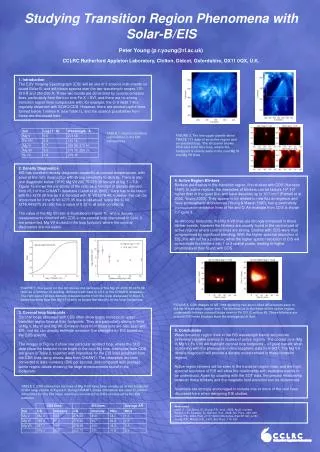
Studying Transition Region Phenomena with Solar-B/EIS

1. Studying Transition Region Phenomena with Solar-B/EIS Peter Young (p.r.young@rl.ac.uk) CCLRC Rutherford Appleton Laboratory, Chilton, Didcot, Oxfordshire, OX11 0QX, U.K. 1. Introduction The EUV Imaging Spectrograph (EIS) will be one of 3 science instruments on board Solar-B, and will obtain spectra over the two wavelength ranges 170-210 Å and 250-290 Å. These two bands are dominated by coronal emission lines, particularly from the iron ions Fe X – XVI, and there are no strong transition region lines comparable with, for example, the O V λ629.7 line regularly observed with SOHO/CDS. However, there are several useful lines formed below 1 million K (see Table 1), and the science possibilities from these are discussed here. TABLE 1. Useful transition region lines in the EIS bandpasses. FIGURE 2. The two upper panels show TRACE 171 data of an active region and an isolated loop. The left panel shows CDS data from this loop, where the footpoint is clearly seen in the cool Mg VI and Mg VII lines 2. Density Diagnostics EIS has excellent density diagnostic capability at coronal temperatures, with several line ratio diagnostics with strong sensitivity to density. There is also one diagnostic below 106 K: Mg VII 280.75/278.39 formed at log T = 5.8. Figure 1a shows the sensitivity of the ratio as a function of density derived from v5.1 of the CHIANTI database (Landi et al. 2005). Care has to be taken with the λ278.39 line as it is blended with Si VII λ278.44, however this can be accounted for if the Si VII λ275.35 line is observed, since the Si VII λ278.44/λ275.35 ratio has a value of 0.32 in all solar conditions. The value of the Mg VII ratio is illustrated in Figure 1b, where density measurements obtained with CDS in the coronal loop discussed in Sect. 3 are presented. Mg VII is used in the loop footpoint where the coronal diagnostics are not useful. 4. Active Region Blinkers Blinkers are flashes in the transition region, first studied with CDS (Harrison 1997). In active regions, the intensities of blinkers can be factors 103-105 higher than in the quiet Sun and have densities up to 1012 cm-3 (Parnell et al. 2002, Young 2003). They appear to be related to new flux emergence and have photospheric abundances (Young & Mason 1997), being particularly pronounced in emission lines of Ne and O. An example from CDS is shown in Figure 3. As with loop footpoints, the Mg V-VII lines are strongly enhanced in these blinker events, however the blinkers are usually found in the central part of active regions where coronal lines are strong. Studies with CDS were thus compromised by significant blending. With the higher spectral resolution of EIS, this will not be a problem, while the higher spatial resolution of EIS will concentrate the blinkers into 1 or 2 spatial pixels, leading to higher photons/pixel than found with CDS. FIGURE 1. The panel on the left shows the variation of the Mg VII λ280.75/λ278.39 ratio as a function of density, derived from data in v.5.1 of the CHIANTI database. The right panel shows density measurements from the loop discussed in Sect. 3, demonstrating how the Mg VII is able to probe the density in the loop footpoints. FIGURE 3. CDS images of AR 7968 showing two short-lived AR blinkers seen in the Ne VI transition region line. The blinkers lie in the heart of the active region, underneath intense coronal loops seen in Fe XVI (2 million K). These blinkers are around 200 times brighter than the average quiet Sun. 3. Coronal loop footpoints Coronal loops observed with CDS often show bright emission in upper transition region lines at their footpoints. They are particularly strong in lines of Mg V, Mg VI and Mg VII. Emission lines from these ions are also seen with EIS, and we can directly estimate emission line strengths for EIS based on the CDS spectra. The images in Figure 2 show one particular isolated loop, where the CDS data show the footpoint to be bright in the cool Mg ions. Intensities from CDS are given in Table 2, together with intensities for the EIS lines predicted from the CDS lines using atomic data from CHIANTI. The intensities are then converted to data numbers (DN) per second, and compared with average active region values showing the large enhancements found in the footpoints. 5. Conclusions Weak transition region lines in the EIS wavelength bands will provide extremely valuable science in studies of active regions. The coolest ions (Mg V, Mg VI, Fe VIII) will highlight coronal loop footpoints – of great benefit when combining with the photospheric/chromospheric data from SOT. The Mg VII density diagnostic will provide a density measurement in these footpoint regions. Active region blinkers will be seen in the transition region lines, and the high spectral resolution of EIS will allow the relationship with explosive events to be understood. Again by coupling with the SOT data, the precise relationship between these blinkers and the magnetic field evolution can be determined. Scientists are strongly encouraged to include one or more of the cool lines discussed here when designing EIS studies. TABLE 2. CDS intensities for lines of Mg V-VII have been measured at the footpoint of the loop shown in Figure 2. Using CHIANTI, these intensities are used to predict intensities for the EIS lines, which are converted to DN/s measured by the EIS detector. References Landi, E., Del Zanna, G., Young, P.R., et al., 2005, ApJS, in press Parnell, C.E., Bewsher, D., Harrison, R.A., 2002, Sol. Phys., 206, 249 Young, P.R., 2004, Proc. of 13th SOHO Workshop, ESA SP-547, p.257 Young, P.R., Mason, H.E., 1997, Sol. Phys., 175, 523