Download
1 / 66
660 likes | 735 Views
Explore solutions for higher field regions between support cylinders and field cages, using SolidWorks Simulator for electric field calculations with analogous thermal Finite Element Analysis (FEA). The study involves verification, shroud geometries, termination joints, testing setups, and elimination of insulating layers. Achieved field accuracy is better than 3 significant figures. The research focuses on grounded shroud options and various joint methods, contributing to better field control and safety in the resistor chain. Calculations demonstrate maximum field capacitors tested, joint variations, and resistor chain covers.

E N D
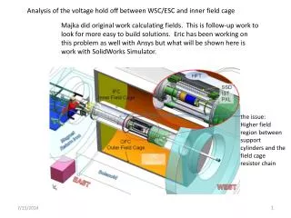
Analysis of the voltage hold off between WSC/ESC and inner field cage Majka did original work calculating fields. This is follow-up work to look for more easy to build solutions. Eric has been working on this problem as well with Ansys but what will be shown here is work with SolidWorks Simulator. the issue: Higher field region between support cylinders and the field cage resistor chain
Old Shroud Design with IDS for FGT only installation conductive composite at ground potential fiber glass insulator plus maybe Mylar conductive surface biased to – 5.5 kV
Calculations of electric fields with analogous thermal FEA • Verification of code with concentric cylinder geometry • Electric field calculations for some shroud geometries and joints • Electric field for biased shroud termination with field grading rings • Electric field calculations for some testing setups (these are for some physical tests of shroud designs and materials)
Calculations of electric fields with analogous thermal FEA Our version of SolidWorks Simulation (FEA code) does not do Electric fields, but it does do thermal conduction through solid materials. The math is the same for either case and we can equate fixed temperature boundary conditions to fixed electric potential boundary conditions. The electric field is equated to temperature gradient. For electrostatic calculations with different dielectrics this can be handled using materials with appropriate ratios of thermal conductivity. In principle sources of heat flux in the thermal code could be used to represent electric charge, but we have not done this in the following work. There is a significant advantage in using the SolidWorks Simulation because of the ease of handling geometries and boundary conditions. The package is tightly integrated which facilitates rapid adjustment and changes. Cases with different geometry parameters can often be run with out changes to the FEA portion.
10000 V Test of SolidWorks Simulator Field Calculation using thermal analog for concentric cylinders r=2 cm (default mesh) r = .11 cm 0 V outer cylinder radius: b inner cylinder radius: a
exchange deg C for Volts Example output for numbers above
Test of SolidWorks Field Calculation With concentric cylinders (using mesh control) .04 cm mesh control set to .01 cm inner surface. default was .027 cm
Conclusion: Field accuracy achieved with SolidWorks Simulator is better than 3 significant figures
The following explores grounded shroud options using a variety of methods for joining the shroud with the WSC/ESC. Different shroud geometries are also explored. Using a grounded shroud as opposed to a biased shroud eliminates the need for a large area insulating layer and it avoids problems of edge termination. Most of the cases give a maximum field on the resistor chain of 5.7 kV/cm. This over a limited area and should be acceptable since we are currently running with 5.6 kV/cm between the gas vessel and the outer field cage. Fields are calculated with SolidWorks Simulator using a thermal analog.
Air_sh_out_hoop1.SLDPRT Case 1 hoop joint joining shroud pieces at 30.8 cm from the center, i.e. 17800 bias on the resistor chain cover shown on this side. max field on the resistor cover: 5.3 kV/cm resistor side, note slight increase in the field where the resistor chain cover passes over the hoop bump
Case 1 Air_sh_out_hoop1.SLDPRT
Case 1 cross section of hoop that covers seam between shroud sections Air_sh_out_hoop1.SLDPRT
Case 1 Air_sh_out_hoop1.SLDPRT
Air_sh_out_rolled_joint1.SLDPRT Case 2 3mm radius joint joint 76.7 cm from center, i.e. 17800 bias knuckle butt joint Air_sh_out_rolled_joint1.SLDPRT
Case 2 maximum field on joint 4.5 kV/cm Air_sh_out_rolled_joint1.SLDPRT
Case 2 Air_sh_out_rolled_joint1.SLDPRT
Case 2 Air_sh_out_rolled_joint1.SLDPRT
offset one side of the joint radially by 0.5 mm and in z by 0.5 mm This increased max field from 4.5 kV/cm to 5.1 kV/cm max field on the high edge: 5.1 kV/cm max field on the low edge: 4.7 kV/cm Case 3 max field point on the resistor chain side Air_sh_out_rolled_joint2.SLDPRT
Case 3 offset joint geometry Air_sh_out_rolled_joint2.SLDPRT
Shroud coupled to support cylinder without a joint perturbation. Can’t actually build a joint free geometry like this. Case 4 20.7 kV on resistor chain surface 2 cm radius where the shroud breaks over the edge WSC_sol.SLDPRT
Case 4 WSC_sol.SLDPRT
More rounded shroud geometry Case 5 simplified shroud shape: cone cut plus fillets main radius 90 mm WSC_sol2.SLDPRT
Case 5 WSC_sol2.SLDPRT
Rounded shroud geometry with joint Case 6 shroud and WSC 3 mm radius filets at joints WSC_sol3.SLDPRT
Case 6 air 3 mm radius filets at joints WSC_sol3.SLDPRT
Case 6 WSC_sol3.SLDPRT
Case 6 WSC_sol3.SLDPRT
Case 7 6 mm radius joints at WSC – Flange- Shroud WSC_sol4.SLDPRT
Case 7 WSC_sol4.SLDPRT
Case 7 WSC_sol4.SLDPRT
Case 7 WSC_sol4.SLDPRT
Case 7 WSC_sol4.SLDPRT
Case 8 6 mm radius joints with 0.5 mm offset exposure WSC_sol5.SLDPRT
Case 8 WSC_sol5.SLDPRT
Case 8 WSC_sol5.SLDPRT
Case 8 WSC_sol5.SLDPRT
Case 8 WSC_sol5.SLDPRT
Case 8 Surface field at the joint on the flat WSC_sol5.SLDPRT
Case 8 WSC_sol5.SLDPRT
Case 8 WSC_sol5.SLDPRT
cases run best case
Graded strip E field calculation using SolidWorks Simulator with Thermal Analog – air and dielectric insulator • Using thermal conductivity to mock dielectric constants and surface temperatures to define conductive surfaces.
Electric field for a graded structure using thermal analogue 1 cm top 2 kV bottom 0 kV 1 kV 0.8 kV 0.6 kV 0.4 kV 0.2 kV 0.3 cm 0.3 cm dielectric/grade test.SLDASM
conductor air dielectric R 0.0050 cm 0.0254 cm ( 10 mil ) 0.0250 cm To simulate conductor, dielectric and air used different values for thermal conductivity. This may or may not be correct, but choose the following values air 0.53 W/(mK) to be dielectric constant of 1 dielectric 1.749 W/(mK) this is 3.3 times value used for air or dielectric constant of 3.3 i.e. dielectric to be Mylar with dielectric constant of 3.3
Analysis done both as 3D and 2D. 3D takes ~2 minutes and 2D takes ~ 2 seconds. read Celsius as kV 2D 1 kV : 1 deg C dielectric2/grade test2.SLDASM
electric field strength 1 kV/cm : 1 deg C/cm 2D