Kalman Filters
E N D
Presentation Transcript
Kalman Filters ELE 774 - Adaptive Signal Processing
Introduction • Mathematical formulation is described by state space concepts. • Solution is computed recursively. • Both stationary and also non-stationary environments. • Each updated estimate of the state computed from • The previous estimate, and • The new input data (innovation). • A unifying framework for the family of recursive least-squares (RLS) filters. ELE 774 - Adaptive Signal Processing
Recursive MMS Estimation for Scalar RVs • Assume a complete set of observed r.v.s upto time n-1 y(1), y(2), ..., y(n-1) • Let the minimum mean-square estimate of the zero mean x(n-1) be where is the space spanned by the observations y(1) ... y(n-1). • Let there be a new observation y(n), • We estimate x(n) using the observations y(1), y(2),...,y(n-1), y(n) • Do this either by storing y(1), y(2),...,y(n-1) and redo the whole problem, or • Exploit and use the new observation y(n), i.e. use a recursive estimation procedure. ELE 774 - Adaptive Signal Processing
Recursive MMS Estimation for Scalar RVs • What is new in the new observation y(n)? Innovations! • Define the forward prediction error • Prediction order (n-1) increases linearly with n. • According to principle of orthogonality, • fn-1(n) is orthogonal to y(1), y(2), ..., y(n-1). • fn-1(n)is a measure of the new information in y(n) ═>innovations! • Information provided by y(n) is composed of two parts • One that in not new, contained in • One that is new, contained in one-step prediction of y(n) ELE 774 - Adaptive Signal Processing
Recursive MMS Estimation for Scalar RVs • Refer to the prediction error as innovations, and define • Properties of the innovation a(n): • Property 1: a(n) is orthogonal to the observations y(1), y(2), ...,y(n-1) Follows from the principle of orthogonality. • Property 2: a(1), a(2), ..., a(n) are orthogonal to each other Innovations process is white. Follow from ELE 774 - Adaptive Signal Processing
Recursive MMS Estimation for Scalar RVs • Property 3: There is one to one correspondence between One sequence may be obtained from the other by means of a causal and causally invertible filter without any loss of information. To show this use Gram-Schmidt orthogonalization procedure: ELE 774 - Adaptive Signal Processing
Recursive MMS Estimation for Scalar RVs • Collecting all terms together • kth row of the matrix gives the coefficients of the forward prediction-error filter of order k-1. • The innovations can be calculated from the observations, or • The observations can be calculated from the innovations • There is no loss of information in this transformation. ELE 774 - Adaptive Signal Processing
Recursive MMS Estimation for Scalar RVs means or, equivalently ELE 774 - Adaptive Signal Processing
Recursive MMS Estimation for Scalar RVs • Clearly, • Recalling that innovations are orthogonal to each other, and choosing bk to minimize the mean-square estimation error we get • Now rewrite • Adding a correction term bna(n) to the previous estimate gives the updated estimate , can be calculated recursively. ELE 774 - Adaptive Signal Processing
Recursive MMS Estimation for Scalar RVs • Predictor – Corrector structure • The use of observations to compute a forward prediction error – innovations, • The use of the innovation to update (correct) the minimum mean-square estimate of a r.v. related linearly to the observations ELE 774 - Adaptive Signal Processing
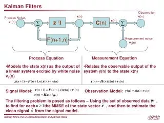
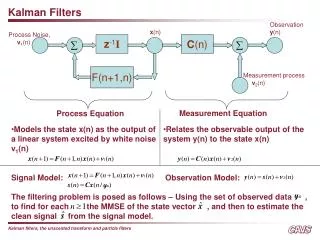
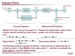
Process Equation Measurement Equation Discrete-Time Dynamical System • A linear discrete-time dynamical system can be characterized by ELE 774 - Adaptive Signal Processing
Discrete-Time Dynamical System • The state vector, x(n), is the minimal set of data that is sufficient to uniquely describe the unforced dynamical behaviour of the system. • fewest data on the past behaviour needed to predict the future one. • Dimension M. • The observation vector, y(n), is the set of observed data. • Dimension N. ELE 774 - Adaptive Signal Processing
Discrete-Time Dynamical System Transition matrix • The process equation: • models an unknown physical stochastic phenomenon denoted by the state x(n) as the output of a linear dynamical systemexcited by the white noise n1(n). • Properties of the transition matrix • 1. Product rule • 2. Inverse rule • Corollary ELE 774 - Adaptive Signal Processing
Discrete-Time Dynamical System • The measurement equation • gives the relation between the state x(n) and the output y(n), with zero-mean white measurement noise (disturbance) n2(n) • Initial value of the state : x(0) • uncorrelated with both n1(n) and n2(n), • Noise vectors n1(n) and n2(n) are statistically independent ELE 774 - Adaptive Signal Processing
Process Equation Measurement Equation Kalman Filtering • We need to solve these eqn.s jointly to find the state x(n) • Use the entire observed data, • consisting of the observations y(1), y(2), ..., y(n) • to find the minimum mean-square estimate of the statex(i), n ≥ 1 • i = n, filtering, • i > n, prediction, • i < n, smoothing. ELE 774 - Adaptive Signal Processing
The Innovations Process • Let the MMS estimate of y(n) be • Span of the vector space is y(1), y(2), ..., y(n-1) • The innovations process associated with y(n) • (Similar to the scalar case) • the Mx1 vector a(n) represents the new information in the observed data y(n). ELE 774 - Adaptive Signal Processing
The Innovations Process • Properties of the innovations process: • Property I: • a(n) is orthogonal to all past observationsy(1), ..., y(n-1) • Property II: • The innovations process consists of a sequence of vector random variables that are orthogonal to each other • Property III: • There is a one-to-one correspondence between the observations and the observation process. One sequence may be obtained from the other by means of linear stable operators, without loss of information. ELE 774 - Adaptive Signal Processing
The Innovations Process • Correlation Matrix of the Innovations Process • Starting from initial state (n=0), we write • i.e. x(k) is a linear combination of x(0), n1(1), ..., n1(k-1) • We know that , then • 1. • 2. • 3. ELE 774 - Adaptive Signal Processing
The Innovations Process • Recall that • Then, given the past decisions , i.e. , the MMS estimate of y(n) • Hence • Predicted state-error vector at time n using data up to time n-1. ELE 774 - Adaptive Signal Processing
The Innovations Process • Autocorrelation of the innovation processa(n) where the predicted state-error correlation matrix is • statistical description of the error in the predicted estimate ELE 774 - Adaptive Signal Processing
Estimation of the State • Minimum mean-square estimation of the state x(n) • Estimate may be expressed as a linear combination of the sequence of innovations process: • Using principle of orthogonality ELE 774 - Adaptive Signal Processing
Estimation of the State • Minimum mean-square estimate of x(n) • Let i=n+1 ELE 774 - Adaptive Signal Processing
Estimation of the State • Summation in is • Then • Kalman Gain • Define • Then ELE 774 - Adaptive Signal Processing
Estimation of the State • Convenient way to calculate the Kalman gain • Hence,Kalman gain becomes • Rewriting the estimate have to be calculated at each iteration! Let’s make it recursive. ELE 774 - Adaptive Signal Processing
Estimation of the State • Kalman gain computer ELE 774 - Adaptive Signal Processing
Estimation of the State • Riccati Equation: • Predicted state-error vector: • After substitution and manipulations ELE 774 - Adaptive Signal Processing
Estimation of the State • We want to find K(n,n-1), hence from previous slide • Then using (1) and (2), we get the Riccati difference equation where ELE 774 - Adaptive Signal Processing
Estimation of the State • Riccati equation solver ELE 774 - Adaptive Signal Processing
Estimation of the State • Kalman’s one-step prediction algorithm: ELE 774 - Adaptive Signal Processing
Estimation of the State • One step prediction algorithm ELE 774 - Adaptive Signal Processing
Filtering • Compute the filtered estimate by using the one-step prediction algorithm. • The state x(n) and the process noise n1(n) are independent of each other. • The MMSE estimate x(n+1) given the observations upto time n is where second line follows from the fact that y(n) and n1(n) are independent of each other. ELE 774 - Adaptive Signal Processing
Filtering • Filtered Estimation Error and Conversion Factor • Define the filtered estimation error vector • We know that • Then Conversion factor ELE 774 - Adaptive Signal Processing
Filtering • Substituting gives • Filtered State-Error Correlation Matrix • Definefiltered state-error vector ELE 774 - Adaptive Signal Processing
Filtering • Manipulations give us • Initial Conditions: • Initial state of the process equation is not precisely known • In the absence of any observed data at n=0, let and if x is zero mean and ELE 774 - Adaptive Signal Processing
Filtering • Kalman filter based on one-step prediction ELE 774 - Adaptive Signal Processing
Summary ELE 774 - Adaptive Signal Processing