Download
1 / 23
250 likes | 620 Views
Introduction to Kalman Filters. Michael Williams 5 June 2003. Overview. The Problem – Why do we need Kalman Filters? What is a Kalman Filter? Conceptual Overview The Theory of Kalman Filter Simple Example. The Problem. Black Box. System Error Sources.

E N D
Introduction to Kalman Filters Michael Williams 5 June 2003
Overview • The Problem – Why do we need Kalman Filters? • What is a Kalman Filter? • Conceptual Overview • The Theory of Kalman Filter • Simple Example
The Problem Black Box System Error Sources • System state cannot be measured directly • Need to estimate “optimally” from measurements External Controls System System State (desired but not known) Optimal Estimate of System State Observed Measurements Measuring Devices Estimator Measurement Error Sources
What is a Kalman Filter? • Recursive data processing algorithm • Generates optimal estimate of desired quantities given the set of measurements • Optimal? • For linear system and white Gaussian errors, Kalman filter is “best” estimate based on all previous measurements • For non-linear system optimality is ‘qualified’ • Recursive? • Doesn’t need to store all previous measurements and reprocess all data each time step
Conceptual Overview • Simple example to motivate the workings of the Kalman Filter • Theoretical Justification to come later – for now just focus on the concept • Important: Prediction and Correction
Conceptual Overview • Lost on the 1-dimensional line • Position – y(t) • Assume Gaussian distributed measurements y
Conceptual Overview • Sextant Measurement at t1: Mean = z1 and Variance = z1 • Optimal estimate of position is: ŷ(t1) = z1 • Variance of error in estimate: 2x(t1) = 2z1 • Boat in same position at time t2 - Predicted position is z1
Conceptual Overview prediction ŷ-(t2) measurement z(t2) • So we have the prediction ŷ-(t2) • GPS Measurement at t2: Mean = z2 and Variance = z2 • Need to correct the prediction due to measurement to get ŷ(t2) • Closer to more trusted measurement – linear interpolation?
Conceptual Overview prediction ŷ-(t2) corrected optimal estimate ŷ(t2) measurement z(t2) • Corrected mean is the new optimal estimate of position • New variance is smaller than either of the previous two variances
Conceptual Overview • Lessons so far: Make prediction based on previous data - ŷ-, - Take measurement – zk, z Optimal estimate (ŷ) = Prediction + (Kalman Gain) * (Measurement - Prediction) Variance of estimate = Variance of prediction * (1 – Kalman Gain)
Conceptual Overview ŷ(t2) Naïve Prediction ŷ-(t3) • At time t3, boat moves with velocity dy/dt=u • Naïve approach: Shift probability to the right to predict • This would work if we knew the velocity exactly (perfect model)
Conceptual Overview Naïve Prediction ŷ-(t3) ŷ(t2) Prediction ŷ-(t3) • Better to assume imperfect model by adding Gaussian noise • dy/dt = u + w • Distribution for prediction moves and spreads out
Conceptual Overview Corrected optimal estimate ŷ(t3) Measurement z(t3) Prediction ŷ-(t3) • Now we take a measurement at t3 • Need to once again correct the prediction • Same as before
Conceptual Overview • Lessons learnt from conceptual overview: • Initial conditions (ŷk-1 and k-1) • Prediction (ŷ-k , -k) • Use initial conditions and model (eg. constant velocity) to make prediction • Measurement (zk) • Take measurement • Correction (ŷk , k) • Use measurement to correct prediction by ‘blending’ prediction and residual – always a case of merging only two Gaussians • Optimal estimate with smaller variance
Theoretical Basis • Process to be estimated: yk = Ayk-1 + Buk + wk-1 Process Noise (w) with covariance Q zk = Hyk + vk Measurement Noise (v) with covariance R • Kalman Filter Predicted: ŷ-k is estimate based on measurements at previous time-steps ŷ-k = Ayk-1 + Buk P-k = APk-1AT + Q Corrected: ŷk has additional information – the measurement at time k ŷk = ŷ-k + K(zk - H ŷ-k ) K = P-kHT(HP-kHT + R)-1 Pk = (I - KH)P-k
Blending Factor • If we are sure about measurements: • Measurement error covariance (R) decreases to zero • K decreases and weights residual more heavily than prediction • If we are sure about prediction • Prediction error covariance P-k decreases to zero • K increases and weights prediction more heavily than residual
Correction (Measurement Update) Prediction (Time Update) (1) Compute the Kalman Gain (1) Project the state ahead K = P-kHT(HP-kHT + R)-1 ŷ-k = Ayk-1 + Buk (2) Update estimate with measurement zk (2) Project the error covariance ahead ŷk = ŷ-k + K(zk - H ŷ-k ) P-k = APk-1AT + Q (3) Update Error Covariance Pk = (I - KH)P-k Theoretical Basis
Quick Example – Constant Model Black Box System Error Sources External Controls System System State Optimal Estimate of System State Observed Measurements Measuring Devices Estimator Measurement Error Sources
Quick Example – Constant Model Prediction ŷ-k = yk-1 P-k = Pk-1 Correction K = P-k(P-k + R)-1 ŷk = ŷ-k + K(zk - H ŷ-k ) Pk = (I - K)P-k
Quick Example – Constant Model Convergence of Error Covariance - Pk
Quick Example – Constant Model Larger value of R – the measurement error covariance (indicates poorer quality of measurements) Filter slower to ‘believe’ measurements – slower convergence
References • Kalman, R. E. 1960. “A New Approach to Linear Filtering and Prediction Problems”, Transaction of the ASME--Journal of Basic Engineering, pp. 35-45 (March 1960). • Maybeck, P. S. 1979. “Stochastic Models, Estimation, and Control, Volume 1”, Academic Press, Inc. • Welch, G and Bishop, G. 2001. “An introduction to the Kalman Filter”, http://www.cs.unc.edu/~welch/kalman/