Probabilistic Robotics: Kalman Filters
700 likes | 933 Views
Probabilistic Robotics: Kalman Filters. Sebastian Thrun & Alex Teichman Stanford Artificial Intelligence Lab.

Probabilistic Robotics: Kalman Filters
E N D
Presentation Transcript
Probabilistic Robotics: Kalman Filters Sebastian Thrun & Alex Teichman Stanford Artificial Intelligence Lab Slide credits: Wolfram Burgard, Dieter Fox, Cyrill Stachniss, Giorgio Grisetti, Maren Bennewitz, Christian Plagemann, Dirk Haehnel, Mike Montemerlo, Nick Roy, Kai Arras, Patrick Pfaff and others
Bayes Filter Reminder • Prediction • Measurement Update
m Univariate -s s m Multivariate Gaussians
Multivariate Gaussians • We stay in the “Gaussian world” as long as we start with Gaussians and perform only linear transformations.
Discrete Kalman Filter Estimates the state x of a discrete-time controlled process that is governed by the linear stochastic difference equation with a measurement
Components of a Kalman Filter Matrix (nxn) that describes how the state evolves from t to t-1 without controls or noise. Matrix (nxl) that describes how the control ut changes the state from t to t-1. Matrix (kxn) that describes how to map the state xt to an observation zt. Random variables representing the process and measurement noise that are assumed to be independent and normally distributed with covariance Rt and Qt respectively.
Linear Gaussian Systems: Initialization • Initial belief is normally distributed:
Linear Gaussian Systems: Dynamics • Dynamics are linear function of state and control plus additive noise:
Linear Gaussian Systems: Observations • Observations are linear function of state plus additive noise:
Kalman Filter Algorithm • Algorithm Kalman_filter( mt-1,St-1, ut, zt): • Prediction: • Correction: • Returnmt,St
Prediction • Observation • Correction • Matching Kalman Filter Algorithm
Prediction The Prediction-Correction-Cycle
Correction The Prediction-Correction-Cycle
Prediction Correction The Prediction-Correction-Cycle
Kalman Filter Summary • Highly efficient: Polynomial in measurement dimensionality k and state dimensionality n: O(k2.376 + n2) • Optimal for linear Gaussian systems! • Most robotics systems are nonlinear!
Nonlinear Dynamic Systems • Most realistic robotic problems involve nonlinear functions
EKF Linearization: First Order Taylor Series Expansion • Prediction: • Correction:
EKF Algorithm • Extended_Kalman_filter( mt-1,St-1, ut, zt): • Prediction: • Correction: • Returnmt,St
Localization “Using sensory information to locate the robot in its environment is the most fundamental problem to providing a mobile robot with autonomous capabilities.” [Cox ’91] • Given • Map of the environment. • Sequence of sensor measurements. • Wanted • Estimate of the robot’s position. • Problem classes • Position tracking • Global localization • Kidnapped robot problem (recovery)
EKF_localization ( mt-1,St-1, ut, zt,m):Prediction: Jacobian of g w.r.t location Jacobian of g w.r.t control Motion noise Predicted mean Predicted covariance
EKF_localization ( mt-1,St-1, ut, zt,m):Correction: Predicted measurement mean Jacobian of h w.r.t location Pred. measurement covariance Kalman gain Updated mean Updated covariance
EKF Summary • Highly efficient: Polynomial in measurement dimensionality k and state dimensionality n: O(k2.376 + n2) • Not optimal! • Can diverge if nonlinearities are large! • Works surprisingly well even when all assumptions are violated!
EKF Localization Example • Line and point landmarks
EKF Localization Example • Line and point landmarks
EKF Localization Example • Lines only (Swiss National Exhibition Expo.02)
UKF Sigma-Point Estimate (2) EKF UKF
UKF Sigma-Point Estimate (3) EKF UKF
Unscented Transform Sigma points Weights Pass sigma points through nonlinear function Recover mean and covariance