Download
1 / 19
200 likes | 236 Views
Learn about observers in uncertain environments and the Kalman Filter for optimal estimation. Topics include Gaussian distributions, weighted averages, predictor-corrector methods, dynamic corrections, and Kalman gain.

E N D
Lecture 10:Observers and Kalman Filters CS 344R: Robotics Benjamin Kuipers
Stochastic Models of anUncertain World • Actions are uncertain. • Observations are uncertain. • i ~N(0,i) are random variables
Observers • The state x is unobservable. • The sense vector y provides noisy information about x. • An observer is a process that uses sensory history to estimate x. • Then a control law can be written
Estimates and Uncertainty • Conditional probability density function
Gaussian (Normal) Distribution • Completely described by N(,) • Mean • Standard deviation , variance 2
The Central Limit Theorem • The sum of many random variables • with the same mean, but • with arbitrary conditional density functions, converges to a Gaussian density function. • If a model omits many small unmodeled effects, then the resulting error should converge to a Gaussian density function.
Estimating a Value • Suppose there is a constant value x. • Distance to wall; angle to wall; etc. • At time t1, observe value z1 with variance • The optimal estimate is with variance
A Second Observation • At time t2, observe value z2 with variance
Update Mean and Variance • Weighted average of estimates. • The weights come from the variances. • Smaller variance = more certainty
From Weighted Averageto Predictor-Corrector • Weighted average: • Predictor-corrector: • This version can be applied “recursively”.
Predictor-Corrector • Update best estimate given new data • Update variance:
Static to Dynamic • Now suppose x changes according to
Dynamic Prediction • At t2 we know • At t3 after the change, before an observation. • Next, we correct this prediction with the observation at time t3.
Dynamic Correction • At time t3 we observe z3 with variance • Combine prediction with observation.
Qualitative Properties • Suppose measurement noise is large. • Then K(t3) approaches 0, and the measurement will be mostly ignored. • Suppose prediction noise is large. • Then K(t3) approaches 1, and the measurement will dominate the estimate.
Kalman Filter • Takes a stream of observations, and a dynamical model. • At each step, a weighted average between • prediction from the dynamical model • correction from the observation. • The Kalman gain K(t) is the weighting, • based on the variances and • With time, K(t) and tend to stabilize.
Simplifications • We have only discussed a one-dimensional system. • Most applications are higher dimensional. • We have assumed the state variable is observable. • In general, sense data give indirect evidence. • We will discuss the more complex case next.