Download
1 / 22
220 likes | 383 Views
Ensemble Kalman Filters for WRF-ARW. Chris Snyder MMM and IMAGe National Center for Atmospheric Research Presented by So-Young Ha (MMM/NCAR). Preliminaries. Notation: x = model ’ s state w.r.t. some discrete basis, e.g. grid-pt values

E N D
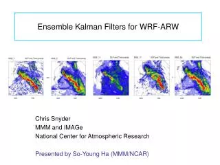
Ensemble Kalman Filters for WRF-ARW Chris Snyder MMM and IMAGe National Center for Atmospheric Research Presented by So-Young Ha (MMM/NCAR)
Preliminaries • Notation: • x = model’s state w.r.t. some discrete basis, e.g. grid-pt values • y = Hx + = vector of observations with random error • Superscript f denotes forecast quantities, superscript a analysis, e.g. xf • Pf = Cov(xf) = forecast covariance matrix … a.k.a. B in Var
Ensemble Kalman Filter (EnKF) • EnKF analysis step • As in KF analysis step, but uses sample (ensemble) estimates for covariances • e.g. one element of PfHT is Cov(xf ,yf) = Ne-1∑(xif - mean(x))(yif - mean(yf)) where yf= Hxf is the forecast, or prior, observation. • Output of EnKF analysis step is ensemble of analyses • EnKF forecast step • Each member integrated forward with full nonlinear model • Monte-Carlo generalization of KF forecast step
Relation of Var and KF … as long as Pf and R are the same in both systems
How the EnKF works • Suppose we wish to assimilate an observation of vr • Consider how assimilation affects a model variable, say w. • Begin with: • ensemble of short-range forecasts (of model variables) • Observed value of vr
How the EnKF works (cont.) • 1. Compute vr for each ensemble member
w vr How the EnKF works (cont.) • 1. Compute vr for each ensemble member
w vr How the EnKF works (cont.) • 1. Compute vr for each ensemble member Ensemble mean
w vr How the EnKF works (cont.) • 1. Compute vr for each ensemble member Ensemble mean Observed value
w vr How the EnKF works (cont.) • 2. Compute best-fit line that relates vr and w
w vr How the EnKF works (cont.) • 3. Analysis moves toward observed value of vr and along best-fit line Analysis (ensemble mean)
w vr How the EnKF works (cont.) • 3. Analysis moves toward observed value of vr and along best-fit line • … have gained information about unobserved variable, w Analysis (ensemble mean)
How the EnKF works (cont.) • 4. Update deviation of each ensemble member about the mean as well. • Yields initial conditions for ensemble forecast to time of next observation.
Flavors of EnKF • ETKF • Pf is sample covariance from ensemble • Analysis increments lie in ensemble subspace • Computationally cheap--reduces to Ne x Ne matrices • Useful for EF but not for DA: In Var “hybrid” system, ETKF updates ensemble deviations but not ensemble mean • “Localized” EnKF • Cov(y,x) assumed to decrease to zero at sufficient distances • Reduces computations and allows increments outside ensemble subspace • approximate equivalence with -CV option in Var--different way of solving same equations • Numerous variants; DART provides several with interfaces for WRF
Data Assimilation Research Testbed (DART) • DART is general software for ensemble filtering: • Assimilation scheme(s) are independent of model • Interfaces exist for numerous models: WRF (including global and single column), CAM (spectral and FV), MOM, ROSE, others • See http://www.image.ucar.edu/DAReS/DART/ • Parallelization • Forecasts parallelized at script level as separate jobs; also across processors, if allowed by OS • Analysis has generic parallelization, independent of model and grid structure
WRF/DART • Consists of: • Interfaces between WRF and DART (e.g. translate state vector, compute distances, …) • Observation operators • Scripts to generate IC ensemble, generate LBC ensemble, advance WRF • Easy to add fields to state vector (e.g. tracers, chem species) • Namelist control of fields in state vector • A few external users (5-10) so far
Nested Grids in WRF/DART • Perform analysis across multiple nests simultaneously • Innovations calculated w.r.t. finest available grid • All grid points within localization radius updated D1 D2 . • D3 obs . obs
Var/DART • DART algorithm • First, calculate “observation priors:”H(xf) for each member • Then solve analysis equations • Possible to use Var for H(xf), DART for rest of analysis • Same interface as between Var and ETKF: H(xf) are written by Var to gts_omb_oma files, then read by DART • Allows EnKF within existing WRF/Var framework, and use of Var observation operators with DART • Under development
Some Applications • Radar assimilation for convective scales • Altug Aksoy (NOAA/HRD) and David Dowell (NCAR) • Assimilation of surface observations • David Dowell and So-Young Ha • Also have single-column version of WRF/DART from Josh Hacker (NCAR) • Tropical cyclones • Ryan Torn (SUNY-Albany), Yongsheng Chen (York), Hui Liu (NCAR) • GPS occultation observations • Liu
References • Bengtsson T., C. Snyder, and D. Nychka, 2003: Toward a nonlinear ensemble filter for high-dimensional systems. J. Geophys. Res., 62(D24), 8775-8785. • Dowell, D., F. Zhang, L. Wicker, C. Snyder and N. A. Crook, 2004: Wind and thermodynamic retrievals in the 17 May 1981 Arcadia, Oklahoma supercell: Ensemble Kalman filter experiments. Mon. Wea. Rev., 132, 1982-2005. • Snyder, C. and F. Zhang, 2003: Assimilation of simulated Doppler radar observations with an ensemble Kalman filter. Mon. Wea. Rev., 131, 1663-1677. • Torn, R. D., G. J. Hakim, and C. Snyder, 2006: Boundary conditions for limited-area ensemble Kalman filters. Mon. Wea. Rev., 134, 2490-2502. • Hacker, J. P., and C. Snyder, 2005: Ensemble Kalman filter assimilation of fixed screen-height observations in a parameterized PBL. Mon. Wea. Rev., 133, 3260-3275. • Caya, A., J. Sun and C. Snyder, 2005: A comparison between the 4D-Var and the ensemble Kalman filter techniques for radar data assimilation. Mon. Wea. Rev., 133, 3081-3094. • Chen, Y., and C. Snyder, 2007: Assimilating vortex position with an ensemble Kalman filter. Mon. Wea. Rev., 135, 1828-1845. • Anderson, J. L., 2007: An adaptive covariance inflation error correction algorithm for ensemble filters. Tellus A, 59, 210-224. • Snyder, C. T. Bengtsson, P. Bickel and J. L. Anderson, 2008: Obstacles to high-dimensional particle filtering. Mon. Wea. Rev., accepted. • Aksoy, A., D. Dowell and C. Snyder, 2008: A multi-case comparative assessment of the ensemble Kalman filter for assimilation of radar observations. Part I: Storm-scale analyses. Mon. Wea. Rev., accepted. • http://www.mmm.ucar.edu/people/snyder/papers/