Download
1 / 52
520 likes | 523 Views
Population sub-structure. Projects. Harish/Nitin Gaurav (Tuesday) Stefano/Hossein (Tuesday) Nisha/Yu David Jian/Josue (Tuesday). Population sub-structure confounds association. Consider an association test in a recently admixed population

E N D
Population sub-structure Structure
Projects • Harish/Nitin • Gaurav (Tuesday) • Stefano/Hossein (Tuesday) • Nisha/Yu • David • Jian/Josue (Tuesday) Structure
Population sub-structure confounds association • Consider an association test in a recently admixed population • Suppose location A increases susceptibility to a disease common in Africans. • Let locus B associate with skin-color. • As expected, locus A is associated with the disease • Unexpectedly, locus B also shows association • The problem arises because the assumption of a random mating population is no longer true • The population has structure! A B 0 .. 1 D 0 .. 1 N 0 .. 0 D 1 .. 1 N 0 .. 1 D 0 .. 1 D 0 .. 1 D 0 .. 1 D 0 .. 1 D African 1 .. 0 N 1 .. 0 N 0 .. 0 D 1 .. 1 D 1 .. 0 N 1 .. 0 N 1 .. 0 N 1 .. 0 N 1 .. 0 N European Structure
Population sub-structure can increase LD Pop. A 0 .. 1 0 .. 1 0 .. 0 1 .. 1 0 .. 1 0 .. 1 0 .. 1 0 .. 1 0 .. 1 p1=0.1 q1=0.9 P11=0.1 D=0.01 Pop. B 1 .. 0 1 .. 0 0 .. 0 1 .. 1 1 .. 0 1 .. 0 1 .. 0 1 .. 0 1 .. 0 p1=0.9 q1=0.1 P11=0.1 D=0.01 • Consider two populations that were isolated and evolving independently. • They might have different allele frequencies in some regions. • Pick two regions that are far apart (LD is very low, close to 0) Structure
Recent ad-mixing of population • If the populations came together recently (Ex: African and European population), artificial LD might be created. • D = 0.15 (instead of 0.01), increases 10-fold • This spurious LD might lead to false associations • Other genetic events can cause LD to increase, and one needs to be careful 0 .. 1 0 .. 1 0 .. 0 1 .. 1 0 .. 1 0 .. 1 0 .. 1 0 .. 1 0 .. 1 Pop. A+B p1=0.5 q1=0.5 P11=0.1 D=0.1-0.25=0.15 1 .. 0 1 .. 0 0 .. 0 1 .. 1 1 .. 0 1 .. 0 1 .. 0 1 .. 0 1 .. 0 Structure
Determining population sub-structure • Given a mix of people, can you sub-divide them into ethnic populations. • Turn the ‘problem’ of spurious LD into a clue. • Find markers that are too far apart to show LD • If they do show LD (correlation), that shows the existence of multiple populations. • Sub-divide them into populations so that LD disappears. Structure
Determining Population sub-structure 0 .. 1 0 .. 1 0 .. 0 1 .. 1 0 .. 1 0 .. 1 0 .. 1 0 .. 1 0 .. 1 1 .. 0 1 .. 0 0 .. 0 1 .. 1 1 .. 0 1 .. 0 1 .. 0 1 .. 0 1 .. 0 • Same example as before: • The two markers are too similar to show any LD, yet they do show LD. • However, if you split them so that all 0..1 are in one population and all 1..0 are in another, LD disappears Structure
Iterative algorithm for population sub-structure • Define • N = number of individuals (each has a single chromosome) • k = number of sub-populations. • Z {1..k}N is a vector giving the sub-population. • Zi=k’ => individual i is assigned to population k’ • Xi,j = allelic value for individual i in position j • Pk,j,l = frequency of allele l at position j in population k Structure
Example • Ex: consider the following assignment • P1,1,0 = 0.9 • P2,1,0 = 0.1 1 1 1 1 1 1 1 1 1 1 2 2 2 2 2 2 2 2 2 2 0 .. 1 0 .. 1 0 .. 0 1 .. 1 0 .. 1 0 .. 1 0 .. 1 0 .. 1 0 .. 1 0 .. 1 P1,1,0 1 .. 0 1 .. 0 0 .. 0 1 .. 1 1 .. 0 1 .. 0 1 .. 0 1 .. 0 1 .. 0 1 .. 0 Structure
Goal • X is known. • P, Z are unknown. • The goal is to estimate Pr(P,Z|X) • Various learning techniques can be employed. • maxP,Z Pr(X|P,Z) (Max likelihood estimate) • maxP,Z Pr(X|P,Z) Pr(P,Z) (MAP) • Sample P,Z from Pr(P,Z|X) • Here a Bayesian (MCMC) scheme is employed to sample from Pr(P,Z|X). We will only consider a simplified version Structure
Algorithm:Structure (Z3,P3) (Z4,P4) (Z2,P2) • Iteratively estimate • (Z(0),P(0)), (Z(1),P(1)),.., (Z(m),P(m)) • After ‘convergence’, Z(m) is the answer. • Iteration • Guess Z(0) • For m = 1,2,.. • Sample P(m) from Pr(P | X, Z(m-1)) • Sample Z(m) from Pr(Z | X, P(m)) • How is this sampling done? (Z1,P1) Structure
Example • Choose Z at random, so each individual is assigned to be in one of 2 populations. See example. • Now, we need to sample P(1) from Pr(P | X, Z(0)) • Simply count • Nk,j,l = number of people in population k which have allele l in position j • pk,j,l = Nk,j,l / N 1 2 2 1 1 2 1 2 1 2 1 2 2 1 1 2 1 2 2 1 0 .. 1 0 .. 1 0 .. 0 1 .. 1 0 .. 1 0 .. 1 0 .. 1 0 .. 1 0 .. 1 0 .. 1 1 .. 0 1 .. 0 0 .. 0 1 .. 1 1 .. 0 1 .. 0 1 .. 0 1 .. 0 1 .. 0 1 .. 0 Structure
Example • Nk,j,l = number of people in population k which have allele l in position j • pk,j,l = Nk,j,l / Nk,j,* • N1,1,0 = 4 • N1,1,1 = 6 • p1,1,0 = 4/10 • p1,2,0 = 4/10 • Thus, we can sample P(m) 1 2 2 1 1 2 1 2 1 2 1 2 2 1 1 2 1 2 2 1 0 .. 1 0 .. 1 0 .. 0 1 .. 1 0 .. 1 0 .. 1 0 .. 1 0 .. 1 0 .. 1 0 .. 1 1 .. 0 1 .. 0 0 .. 0 1 .. 1 1 .. 0 1 .. 0 1 .. 0 1 .. 0 1 .. 0 1 .. 0 Structure
Sampling Z • Pr[Z1 = 1] = Pr[”01” belongs to population 1]? • We know that each position should be in linkage equilibrium and independent. • Pr[”01” |Population 1] = p1,1,0 * p1,2,1 =(4/10)*(6/10)=(0.24) • Pr[”01” |Population 2] = p2,1,0 * p2,2,1 = (6/10)*(4/10)=0.24 • Pr [Z1 = 1] = 0.24/(0.24+0.24) = 0.5 Assuming, HWE, and LE Structure
Sampling • Suppose, during the iteration, there is a bias. • Then, in the next step of sampling Z, we will do the right thing • Pr[“01”| pop. 1] = p1,1,0 * p1,2,1 = 0.7*0.7 = 0.49 • Pr[“01”| pop. 2] = p2,1,0 * p2,2,1 =0.3*0.3 = 0.09 • Pr[Z1 = 1] = 0.49/(0.49+0.09) = 0.85 • Pr[Z6 = 1] = 0.49/(0.49+0.09) = 0.85 • Eventually all “01” will become 1 population, and all “10” will become a second population 1 1 1 2 1 2 1 2 1 1 2 2 2 1 2 2 1 2 2 1 0 .. 1 0 .. 1 0 .. 0 1 .. 1 0 .. 1 0 .. 1 0 .. 1 0 .. 1 0 .. 1 0 .. 1 1 .. 0 1 .. 0 0 .. 0 1 .. 1 1 .. 0 1 .. 0 1 .. 0 1 .. 0 1 .. 0 1 .. 0 Structure
Allowing for admixture • Define qi,k as the fraction of individual i that originated from population k. • Iteration • Guess Z(0) • For m = 1,2,.. • Sample P(m),Q(m) from Pr(P,Q | X, Z(m-1)) • Sample Z(m) from Pr(Z | X, P(m),Q(m)) Structure
Estimating Z (admixture case) • Instead of estimating Pr(Z(i)=k|X,P,Q), (origin of individual i is k), we estimate Pr(Z(i,j,l)=k|X,P,Q) i,1 i,2 j Structure
Results: Thrush data • For each individual, q(i) is plotted as the distance to the opposite side of the triangle. • The assignment is reliable, and there is evidence of admixture. Structure
NJ versus Structure:thrush data • Objective function is different in standard clustering algorithms! Structure
Population Structure in isolated human populations Oceania Eurasia East Asia America Africa • 377 locations (loci) were sampled in 1000 people from 52 populations. • 6 genetic clusters were obtained, which corresponded to 5 geographic regions (Rosenberg et al. Science 2003) Structure
Population sub-structure:research problem • Systematically explore the effect of admixture. Can admixture be predicted for a locus, or for an individual • The sampling approach may or may not be appropriate. Formulate as an optimization/learning problem: • (w/out admixture). Assign individuals to sub-populations so as to maximize linkage equilibrium, and hardy weinberg equilibrium in each of the sub-populations • (w/ admixture) Assign (individuals, loci) to sub-populations Structure
Population Substructure Conclusions • Populations substructure (violating the assumption of random mating) can create artificial linkage disequlibrium, and false associations • One way out of it is to identify and sub-divide the populations into sub-populations. • Another approach is to ‘correct’ for the effects of structure. Structure
Detecting structural variations Structure
Genomic variation • Inherited phenotypes arise from genetic variation • Point mutations, indels, genetic recombination, but also…. • Structural Variation • Insertions, deletions, translocations, inversions, fissions, fusions…. deletions inversions translocations Structure
Fluoroscent in situ hybridization • (Cancer genomes show extensive structural variation) • Historically, larger structural variations (easily observed under a microscope were commonly studied, mostly in the context of diseases… Structure
HapMap and other projects • The development of molecular techniques (sequencing, genotyping) shifted interest onto smaller scale mutations. They were assumed to be the dominant source of genetic variation • It turns out that structural variation in normal populations is more common than assumed. Structure
1. Inversions and HapMap T C A C • SNP data is seemingly oblivious to Inversions (& other structural polymorphisms) • Can we detect a signal for inversion polymorphisms in SNPs? reference genome sequence A A G A A A G G A A G G A A T G G G G G G A G A G G A A A G G A G A population A G T G C T G C A Structure
Array-CGH Garnis et al. Molecular Cancer 2004 Structure
Structural variations • Structural variants are common, but non CNVs are hard to detect. • Some of the translocations are important in disease Structure
2. Variations in tumor genomes • Fusion observed in leukemia, lymphoma, and sarcomas • “Philadelphia Translocation” Drugs target this fusion protein • Can we detect fused genes in tumors? Structure
3. Assaying for specific variations • Most tumors start off with a single cell, which then proliferate. • Drugs like Gleevec are used well after cancer has taken hold. • Can we detect the cancer early by detecting the genomic abnormality? • If a very few cells in the person are cancerous, can we still detect it? • Can we track a patient through his treatment? Structure
Today • Detection of inversion polymorphisms (& other copy neutral variation) using genotype data. • Detection of gene fusion events using sequencing • PCR based detection of variation in the presence of heterosomy: only a fraction of cells carry the variant genome Structure
Chr. 17 Inversion Structure
Inversion polymorphisms Structure
Common inverted haplotype Structure
LLR statistic computation M1 M2 M3 M4 • Multi-allelic markers are chosen in blocks around the putative breakpoints • LD is measured using multi-allelic D-statistic LD12 LD13 LD24 LD34 Bansal et al. Genome Research, 2007 Structure
LLRl d12 d13 M1 M2 M3 M4 LD13 LD13 Structure
LLRR d12 d24 M1 M2 M3 M4 LD24 LD34 Structure
Inversion polymorphisms in human • LLRl and LLRr define our inversion statistic • Large positive values for both likelihood ratios indicate inversion • A permutation test to estimate the significance of the statistic • Overlapping breakpoints are merged Structure
Power • Difficult to simulate inversions using the coalescent • We simulated inversions on HapMap data. • (a) varying frequency, 500kb inversion • (b) varying length Structure
Inversion polymorphisms • We used the Phase I phased haplotype data from the International HapMap project • 3 samples: CEU, YRI, Asian: CHB+JPT about 900K SNPs • The location between two adjacent SNPs was considered a potential inversion breakpoint • The statistic was computed for every pair of inversion breakpoints within a certain distance (200kb - 6Mb) • 176 inversion polymorphisms were detected Structure
Inversions with secondary evidence • 18 regions had highly homologous repeat sequence, 11 with inverted repeats (p-value 0.006 against random distribution of inversion breakpoints) Structure
Inversions with secondary evidence Structure
1.4Mb inversion at 16p12(CEU+YRI) • Supported by fosmid pair evidence (Tuzun et al., 2005) • 80kb long inverted repeat • Identical breakpoints in CEU and YRI data • Known chimp repeat Structure
1.2Mb Chr 10 (CHB+JPT) • Inversion supported by fosmid evidence (Tuzun et al. 2005) Structure
Chr 6 Inversion(YRI) & TCBA1 • 66 inversion breakpoints covered by genes • Less than expected by chance (p-value 0.02) • Many overlapping genes are known to be disrupted in disease • T-cell lymphoma breakpoint associated target (TCBA1) • Structurally disrupted in T-cell lymphoma cell-lines Structure
ICAp69 • Islet cell antigen (ICAp69) gene Structure
Inversion Polymorphism summary • Many inversions (and copy neutral) polymorphisms remain to be detected. • The genotype LD signal is useful but has low power. • We are investigating other signals to improve detection • Some of these variations lead to genes fusing. Structure
Conclusions for the class • Genetic variations are important to our understanding of evolution and genotype-phenotype relationship Structure