Download
1 / 53
620 likes | 810 Views
POPULATION STRUCTURE. 3. 2. 1. POPULATION STRUCTURE. A. A. B. B. POPULATION STRUCTURE. Gene flow (migration*). Low levels of gene flow (migration*). High levels of gene flow (migration*). POPULATION STRUCTURE. Natural selection.

E N D
POPULATION STRUCTURE
3 2 1 POPULATION STRUCTURE A A B B
POPULATION STRUCTURE • Gene flow (migration*) • Low levels of gene flow (migration*) • High levels of gene flow (migration*)
POPULATION STRUCTURE • Natural selection • Genetic drift - random nature of transmitting alleles from one generation to the next • Differences in allele frequencies between the initial founders of the populations
POPULATION STRUCTURE • Genetic drift RIVER (Vicariance)
POPULATION STRUCTURE • Founder effect - a new population is started by a few members of the original population. This small population size means that the population may have: • reduced genetic variation from the original population. • a non-random sample of the genes in the original population.
POPULATION STRUCTURE Some degree of differentiation is maintained in the absence of contemporary barriers to gene flow by little interbreeding due to: • differences in reproductive timing • assortative mating • homing • low dispersal capabilities
1 2 3 Heterozygote deficiency POPULATION STRUCTURE • Potential complications of genetic analysis
WAHLUND EFFECT I If two populations in Hardy-Weinberg equilibrium with different allele frequencies are pooled together cause a deficit of heterozygotes
WAHLUND EFFECT II A and B - populations in HW equilibrium curved line - expected HW frequency line – genotype frequencies resulting from a mixture of the genotypes P – population composed of 50% from each of population A and B (deficit of heterozygotes) F1 – Population P after one generation of random mating aa One generation of random mating in the pooled population will result in Hardy-Weinberg proportions of genotypes
WAHLUND EFFECT III Gadus morhua Sick (1965)
WAHLUND EFFECT V Heterogenous allele frequencies
WAHLUND EFFECT VI Squirrels 48% (He) 24% (He) 8% The frequencies of both homozygotes have decreased by 4% in the fused population compared to their average frequencies in the subdivided populations. In contrast, the frequency of heterozygotes in the fused population increased. 2pqfused = 2(0.2)(0.8) = 0.32
The main effect of the population substructure is a decrease in the proportion of heterozygous genotypes
WRIGHT’S F STATISTICS A subdivided population has three distinct levels of complexity: individuals (I), subpopulations (S) and total population (T). The partitions of heterozygosity: HI – the heterozygosity of an individual in a subpopulation (average heterozygosity of all genes in an individual across subpopulations) HS – expected average heterozygosity in each subpopulation with random mating (HW) HT - expected heterozygosity of an individual in the total population with random mating (HW)
Inbreeding coeficient– reduction in heterozygosity of an individual due to nonrandom mating within its subpopulation. FIS = Hs – Hi / Hs Overall inbreeding coeficient - reduction in heterozygosity of an individual relative to the total population. FIT = HT – Ho / HT Fixation index- reduction in heterozygosity of a subpopulation due to random genetic drift. FST= HT – Hs / HT WRIGHT’S F STATISTICS Estimating F Statistics:
WRIGHT’S F STATISTICS Hs (expected average heterozygosity HW) = (2pqPOP1+2pqPOP2)/2; we need to estimate the frequency of p and q in each population POP1 – p=0.898 q=0.102 2pq=0.183 POP2 – p=0.842 q=0.158 2pq=0.265 Hs = (0.183+0.265)/2= 0.224
WRIGHT’S F STATISTICS HT – expected average heterozygosity in total population HW; we need to estimate the frequency of p and q in the total population (p1+p2)/2 = 0.871 (q1+q2)/2=0.130 POP2 – p=0.842 q=0.158 2pq=0.265 POP1 – p=0.898 q=0.102 2pq=0.183 HT = 2pq=2(0.871) (0.130)/2= 0.226
WRIGHT’S F STATISTICS FST= HT – Hs / HT = (0.226-0.224)/0.226= 0.009 FST < 0.05 low genetic differentiation FST > 0.25 high genetic differentiation
WRIGHT’S F STATISTICS Other ways to estimate F STATISTICS : • Analysis of variance of Cockerham • Bootstrapping techniques Weir and Cockerham
WRIGHT’S F STATISTICS Gst: extension of FST multiple alleles Θst: considers sample size biased Microsatellites (Setpwise mutation model) ASD, (δμ)2, Dsw, Rst : considers the high mutation rates of microsatellites Genetic Distance Nei (1972) – take into account the mutation and drift Cavalli-Sforza and Edwards (1967) – only drift The FST is a measure of genetic differentiation, but there are others:
Differentiation is not the same as Distance Differentiation -considers how genetic diversity is distributed within and among populations Distance – takes into account the sharing of alleles and also the allele frequencies. Fst – measures the effects of population substructure and the reduction of heterozygozity due to the genetic drift B A Distance high (no allele sharing). Diferentiation low (high variability within populations)
Diferentiation VERSUS genetic distance Cl6 Cl39 CL5 Cl19 CL136 Cl17 Cl145 Salas 215 147147 170170 116116 176180 182190 207207 122126 Salas 216 147147 170170 116116 172180 178186 207207 122126 Salas 217 147147 170170 116116 176188 190190 203207 122126 Muradal 423 156159 172174 119137 184204 170174 191195 120134 Muradal 176 159159 172172 143161 192208 166174 191191 120130 Muradal 177 156162 172172 119143 192196 170174 191195 114130 Muradal 178 159162 172172 146158 184196 170170 191195 130130 Weir & Cockerham’s FIS= -0.13744 FIT= 0.39912 FST= 0.47 Distance (Cavalli-Sforza & Edwards) = 0.85
Analysis of Molecular Variance (AMOVA) Method of estimating population differentiation directly from molecular data and testing hypotheses about such differentiation Hierarchical levels of differentiation: • Within populations • Among populations within groups • Among groups
MODELS OF POPULATION STRUCTURE AND GENE FLOW • Study the effects of migration, using simple models of population structure • These general models may not precisely fit a particular biological example, but they give close approximations to many situations and allow an evaluation of the effect of limited gene flow.
Thecontinent-ISLAND MODEL A large population is split into many subpopulations dispersed geographically, like islands in an archipelago or fishes in ponds with a lake as the source of gene flow • Unidirectional gene flow, and drift is neglected (in the large population) • Only gene flow is important to the island
ISLAND MODEL The allele frequency over time in five subpopulations with different initial allele frequencies converge rapidly to a common equilibrium frequency.
WRIGHT’s Island MODEL • gene flow can occur among all subpopulations (bidirectional) FST ≈1/4Nm+1 • differentiation among subpopulations results from an equilibrium between genetic drift (a function of N) and gene flow (m)
Very high divergence High divergence Moderate divergence Low divergence ISLAND MODEL Differentiation as a function of migration
STEPPING STONE MODEL • For organisms with relatively low effective rates of dispersal, most gene exchange will occur between neighboring subpopulations. • Populations are organized in subpopulations with discrete differentiation • Only migration into adjacent subpopulations (e.g This pattern of migration is common for species distributed in linear habitats, such as estuaries along a coast).
STEPPING STONE MODEL II Some of the results provided by this type of model are quite simple and include clines of allelic frequencies along a geographic transect as a result of: Admixture between adjacent populations Isolation by distance Diferencial selection
Gradual changes in allele frequency over geographic distance
ISOLATION BY DISTANCE The genetic correlation between individuals declines as a function of geographic distance between them
ESTIMATING MIGRATION RATES Direct - estimates is extremely difficult Indirect - Methods based on genetic information • FST • Private alleles of Slatkin • Methods based on the Coalescent theory (Island model e Isolation Model)
ESTIMATING MIGRATION RATES Private alleles Slatkin (1985) demosntrated that, The frequency of private alleles in one population is proportionally inverse to Nm Estimates based on ISLAND MODEL Wright (1931) as demonstrated that in equilibrium, Fst=1/(1+4Nm) Nm = (1 – FST) / 4FST FST = 0.009; Nm = 25.7 migrant individuals between populacions per generation
ESTIMATING MIGRATION RATES Limitations: • Constant effective population size • Infinite number of populations • Equilibrium (mutation, drift and gene flow) • Populations with very high levels of gene flow may not present an enough number of private alleles • Overestimation due to retention of ancestral polymorphism
ESTIMATING MIGRATION RATES Methods based on the Coalescent theory (Island Model) Likelihood and Bayesian methods that use Markov Chain Monte Carlo MCMC (p.ex. software MIGRATE) Limitations: • This model assumes that the populations have separated at an infinitely long time ago and the populations are in drift-migration equilibrium • Overestimation due to retention of ancestral polymorphism
According to this model, sharing of polymorphism between populations is due to migration. But……….. A B
Retention of ancestral polymorphism, which may result in overestimates A B
ISOLATION WITH MIGRATION MODEL Migration or ancestral polymorphism? (Hey & Nielsen 2004).
Isolation with Migration Model Estimates gene flow: • between populations with different effective population size; ii) Assimetrical migration rates (including several models); iii) no-equilibrium (gene flow in recently diverged popuations); iv) Distinguish between retention of ancestral polymorphism and gene flow
Bayesian assignment methods • Use genetic information to ascertain population membership of individuals without assuming predefined populations. • The methods operate by minimizing Hardy–Weinberg and linkage disequilibria, and the assignment of each individual genotype to its population of origin is carried out probabilistically • Geographical or no geographical information • Both Individual sampling and “population sampling”
Bayesian assignment methods “Population” sampling Individual sampling