Download
1 / 62
630 likes | 882 Views
Imaging and deconvolution. Sanjay Bhatnagar, NRAO. Plan for the lecture-I. How do we go from the measurement of the coherence function (the Visibilities) to the images of the sky? First half of the lecture: Imaging Measured Visibilities Dirty Image .

E N D
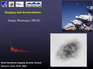
Imaging and deconvolution Sanjay Bhatnagar, NRAO
Plan for the lecture-I • How do we go from the measurement of the coherence function (the Visibilities) to the images of the sky? • First half of the lecture: Imaging • Measured Visibilities Dirty Image •
Second half of the lecture: Deconvolution Dirty image Model of the sky Plan for the lecture-II
Interferometers are indirect imaging devices For small w (small max. baseline) or small field of view (l2 + m2 << 1) I(l,m) is 2D Fourier transform of V(u,v) Imaging
Ideal visibilities(V ) True image(I ) FT This is true ONLY if V is measured for all (u,v)! Imaging: Ideal 2D Fourier relationship
Imaging: UV-plane sampling • With limited number of antennas, the uv-plane is sampled at descrete points: = X VM S Vo
Effect of sampling the uv-plane: Using the Convolution Theorem: The Dirty Image (Id) is the convolution of the True Image (Io) and the Dirty Beam/Point Spread Function (B) B = FT-1(S) In practice Id = B*Io + B*IN where IN = FT-1(Vis. Noise) To recover Io, we must deconvolve B from Id. The algorithm must also separate B*Io from B*IN. Convolution with the PSF
Convolution = I(x0)B(x-xo) + I(x1)B(x-x1) + …
The Dirty Image FT The PSFUV-coverage * The Dirty Image
Fast Fourier Transform (FFT) is used for efficient Fourier transformation. It however requires regularly spaced grid of data. Measured visibilities are irregularly sampled (along uv-tracks). Convolutional gridding is used to effectively interpolate the visibilities everywhere and then re-sample them on a regular grid (the Gridding operation) VS= VM * C = (VoS) * C => Id . FT-1(C) C is designed to have desirable properties in the image domain. Making of the Dirty Image
PSF is a weighted sum of cosines corresponding to the measured fourier components: Visibility weights (wi) are also gridded on a regular grid and FFT used to compute the Dirty Beam (or the PSF). The peak of the PSF is normalized to 1.0 The 'main lobe' has a size Dx ~ 1/umax and Dy~1/vmax This is the 'diffraction limited' resolution (the Clean Beam) of the telescope. Dirty Beam: Interesting properties
Side lobes extend indefinitely RMS ~ 1/N where N = No. of antennas Dirty Beam: Interesting properties
Close-in side lobs of the PSF are controlled by the uv- coverage envelope. E.g., if the envelop is a circle, the side lobes near the main lobe must be similar to the FT of a circle: Bessel function/Radius Close-in side lobes of the PSF
Weighting function (Wk) can be chosen to modify the side lobes Natural Weighting Wk=1/ sk2where sk2is the RMS noise Best RMS across the image. Large scales (smaller baselines) have higher weights. Effective resolution less than the inverse of the longest baseline. PSF forming: Weighting...
Uniform weighting Wk=1/r(uk,vk) where r(uk,vk) is the density of uv-points in the kth cell. Short baselines (large scale features in the image) are weighted down. Relatively better resolution Increases the RMS noise. Super uniform weighting: Consider density over larger region. Minimize side lobes locally. ...Weighting...
Robust/Briggs weighting: Wk= 1/[S.r(uk ,vk) + sk2] Parameterized filter – allows continuous variation between optimal resolution (uniform weighting) and optimal noise (natural weighting). ...Weighting
The PSF can be further controlled by applying a tapering function on the weights (e.g. such that the weights smoothly go to zero beyond the maximum baseline). W'k=T(uk,vk) Wk(uk,vk) Bottom line on weighting/tapering: These help a bit, but imaging quality is limited by the deconvolution process! PSF Forming: Tapering
As seen earlier, not all parts of the uv-plane are sampled – the 'invisible distribution' 1. “Central hole” below uminand vmin: - Image plane effect: Total integrated power is not measured. - Upper limit on the largest scale in the image plane. 2. No measurements beyond umax and vmax: - Size of the main lobe of the PSF is finite (finite resolution). 3. Holes in the uv-plane: - Contribute to the side lobes of the PSF. The missing information
Missing 'central hole' means that the total flux, integrated over the entire image is zero. Total flux for scales corresponding to the fourier components between umax and umin can be measured. In the presence of extended emission, the observations must be designed keeping in mind: - the require resolution ==> maximum baseline - the largest scale to be reliably reconstructed ==> minimum baseline More on missing information
For information beyond the max. baseline, one requires extrapolation. That's un-physical (unconstrained). Information corresponding to the “central hole”: possible, but difficult (need extra information). Information corresponding to the uv-holes: requires interpolation. The measurements provide constraints – hence possible. But non-linear methods necessary. If Z is the unmeasured distribution, then B*Z=0. If IM is a solution to Id=B*IM, then so is IM + aZ for any value of a. Deconvolution = interpolation in the visibility plane. Recovering the missing information
What can we assume about the sky emission: 1. Sky does not look like cosine waves 2. Sky brightness is positive (but there are exceptions) 3. Sky is a collection of point sources (weak assertion) 4. Sky could be smooth 5. Sky is mostly blank (sometimes justifies “boxed” deconvolution) Non-linear deconvolution algorithms search for a model image IM such that the residual visibilities VR=Vo-VM are minimized, subject to the constraints given by the (assumed) prior knowledge. Prior knowledge about the sky
Let A = Measurement matrix to go from the image domain to the visibility domain (the measurement domain). I = Vector of the image pixel values V = Vector of visibilities B = Operator (matrix) for convolution with the PSF N = The noise vector Then, Id = BIo + BIN where BIN = ATAN VM = AIM and Vo = AIo + N VR = Vo – AIM Small digression: Vector notation
A is rectangular (not square) and is a collection of sines and cosines corresponding to only the measured fourier components. A is singular ==> A-1 does not exist IM=A-1VM not possible ==> non-linear methods needed N is independent gaussian random process. Noise in the image domain = BIN Pixel-to-pixel noise in the image is not independent Some observations
For successful recovery of Io given Id, prior knowledge must fundamentally separate BIo and BIN. c2 is the optimal estimator. Deconvolution then is equivalent to: Deconvolution is equivalent to function minimization Algorithms differ in the parameterization of Pk, the type of constraints and the way the constraints are applied. ...more observations
Scale-less algorithms: Popular ones: Clean, MEM and their variants Scale-sensitive algorithms (new turf!): Existing ones: Multi-scale Clean, Asp-Clean Deconvolution algorithms
Prior knowledge: - sky is composed of point sources - mostly blank Algorithm: 1. Search for the peak in the dirty image. 2. Add a fraction g (loop gain) of the peak value to IM. 3. Subtract a scaled version of the PSF from the position of the peak. IRi+1= IRi – g.B.max(IRi) 4. If residuals are not “noise like”, goto 1. 5. Smooth IM by an estimate of the main lobe (the “clean beam”) of the PSF and add the residuals to make the “restored image” The classic Clean algorithm (Hogbom, 1974)
It is a steepest descent minimization. Model image is a collection of delta functions – a scale insensitive algorithm. A least square fit of sinusoids to the visibilities which is proved to converge (Schwarz 1978). Stabilized by keeping a small loop gain (usually g=0.1-0.2). Stopping criteria: either the max. iterations or max. residuals some multiple of the expected peak noise. Search space constrained by user defined windows. Ignores coupling between pixels (extended emission) – assumes an orthogonal search space. Details of Clean
Clean: Model visibilities Model Vis. Sampled Vis Residual Vis. True Vis.
Clark Clean – uses FFT to speed up Minor cycle(inexpensive) : Clean the brightest points using an approximate PSF to gain speed Major cycle(expensive): Use FFT convolution to accurately remove the point sources found in the minor cycle Cotton-Schwab Clean: A variant of Clark Clean Subtract the point sources from the visibilities directly. Sometimes faster and always more accurate then Clark Clean. Easy to adapt for multiple fields. Variants of the Classic Clean
Deconvolution algorithms: MEM • MEM is a constrained minimization algorithm. • Fast non-linear optimization algorithm due to Cornwell&Evans(1983). • Solve the convolution equation, with the constrain of smoothness via the 'entropy' mk is the prior image – usually a flat default image. • Default image is a very useful in incorporating model images from other algorithms etc. • Naturally useful when final image is some combination of images (like mosaic images).
Works better than Clean for extended emission. Every pixel is treated as a potential degree of freedom – a scale insensitive algorithm. Point sources are a problem, particularly along with large scale background emission – but can be removed with, say, Clean before hand. Easier to analyze and understand. MEM: Some points
MEM: Model visibilities Model Vis. Sampled Vis Residual Vis. True Vis.
Limit the search for components to only parts of the image. A way to regularize the deconvolution process. Useful when small no. of visibilities (e.g. VLBI/snapshots). Do not over-Clean within the boxes (over-fitting). Deeper Clean with no/loose boxes and lower loop gain can achieve similar (more objective) results. Stop when Cleaning with in the boxes has no global effect (insignificant coupling of pixels due to the PSF). Role of boxes
Each pixel is not an independent degree of freedom (DOF). E.g., a gaussian shaped source covering 100 pixels can be represented by 5 parameters. Clean/MEM treats each pixel within a clean-box as an independent degree of freedom. Scale fundamentally separates noise and signal. - Largest coherent scale in BIN ~ the size of the resolution element. - Physically plausible IM is composed of scales >= the resolution element (smallest scale is of the size of the resolution element). Scale-sensitive reconstruction therefore leaves more noise-like (uncorrelated) residuals. Fundamenal problem with scale-less decomposition
Inspired by the Clean algorithm (Cornwell&Holdaway). Decompose the image into a pre-computed set of symmetric “blobs” at a few scales (e.g. Gaussians). Algorithm 1. Make residual images smoothed to a few scales. 2. Find the peak among these residual images. 3. Subtract from all residual images a blob of scale corresponding to the scale of the residual image which had the peak. 4. Add the blob to the model image. 5. If more peaks in the residual images, goto 1. 6. Smooth the model image by the “clean beam” and add the residuals. Scale Sensitive Deconvolution: MS-Clean
Deals with compact as well as extended emission better (need to include a blob of zero scale). Retains the scale-shift-n-subtract nature of Clean – easy to implement. Reasonably fast (for what it does!) Breaks up non-symmetric structures (as in Clean – but the errors are at larger scales than in Clean). Ignores coupling between blobs. Assumes an orthogonal space and steepest descent minimization. MS-Clean details
MS-Clean: Model visibilities Model Vis. Sampled Vis Residual Vis. True Vis.