Download
1 / 24
240 likes | 253 Views
Image deconvolution, denoising and compression. T.E. Gureyev and Ya.I.Nesterets 15.11.2002. CONVOLUTION.

E N D
Image deconvolution, denoising and compression T.E. Gureyev and Ya.I.Nesterets 15.11.2002
CONVOLUTION where D(x,y) is the experimental data (registered image),I(x,y) is the unknown "ideal" image (to be found),P(x,y) is the (usually known) convolution kernel,* denotes 2D convolution, i.e. and N(x,y) is the noise in the experimental data. In real-life imaging, P(x,y) can be the point-spread function of an imaging system; noise N(x,y) may not be additive. Poisson noise:
EXAMPLE OF CONVOLUTION = * 3% Poisson noise 10% Poisson noise
DECONVOLUTION PROBLEM Deconvolution problem: given D, P and N, find I(i.e. compensate for noise and the PSF of the imaging system) Blind deconvolution: P is also unknown. Equation (*) is mathematically ill-posed, i.e. its solution may not exist, may not be unique and may be unstable with respect to small perturbations of "input" data D, P and N. This is easy to see in the Fourier representation of eq.(*) 1) Non-existence: 2) Non-uniqueness: 3) Instability:
A SOLUTION OF THE DECONVOLUTION PROBLEM Convolution: Deconvolution: We assume that (otherwise there is a genuine loss of information and the problem cannot be solved). Then eq.(!) provides a nice solution at least in the noise-free case (as in reality the noise cannot be subtracted exactly). (*)-1 =
NON-LOCALITY OF (DE)CONVOLUTION The value of convolution I*P at point (x,y) depends on all those values I(x',y') within the vicinity of (x,y) whereP(x-x', y-y')0. The same is true for deconvolution. Convolution with a single pixel wide mask at the edges Deconvolution (the error is due to the non-locality and the 1-pixel wide mask)
EFFECT OF NOISE In the presence of noise, the ill-posedness of deconvolution leads to artefacts in deconvolved images: The problem can be alleviated with the help of regularization without regularization = (*)-1 3% noise in the experimental data with regularization
EFFECT OF NOISE. II In the presence of stronger noise, regularization may not be able to deliver satisfactory results, as the loss of high frequency information becomes very significant. Pre-filtering (denoising) before deconvolution can potentially be of much assistance. without regularization = (*)-1 10% noise in the experimental data with regularization
DECONVOLUTION METHODS Two broad categories (1) Direct methodsDirectly solve the inverse problem (deconvolution). Advantages: often linear, deterministic, non-iterative and fast. Disadvantages: sensitivity to (amplification of) noise, difficulty in incorporating available a priori information. Examples: Fourier (Wiener) deconvolution, algebraic inversion. (2) Indirect methodsPerform (parametric) modelling, solve the forward problem (convolution) and minimize a cost function. Disadvantages: often non-linear, probabilistic, iterative and slow. Advantages: better treatment of noise, easy incorporation of available a priori information.Examples: least-squares fit, Maximum Entropy, Richardson-Lucy, Pixon
DIRECT DECONVOLUTION METHODS Fourier (Wiener) deconvolutionBased on the formulaRequires 2 FFTs of the input image (very fast)Does not perform very well in the presence of noise Convolution with 10% noise
ITERATIVE WIENER DECONVOLUTION The method proposed by A.W.StevensonBuilds deconvolution as Requires 2 FFTs of the input image at each iterationCan use large (and/or variable) regularization parameter Convolution with 10% noise
Richardson-Lucy (RL) algorithm If PSF is shift invariant then RL iterative algorithm is written as I(i+1)= I(i) Corr(D/ (I(i)P), P) Correlation of two matrices is Corr(g, h)n,m= i jgn+i,m+jhi,j Usually the initial guess is uniform, i.e. I(0) = D • Advantages: • Easy to implement (no non-linear optimisation is needed) • Implicit object size (In(0) = 0 In(i) = 0 i)and positivity constraints (In(0) > 0 In(i) >0 i) • Disadvantages: • Slow convergence in the absence of noise and instability in the presence of noise • Produces edge artifacts and spurious "sources"
No noise RL Original Image Data 1000 RL iterations 50 RL iterations
3% noise RL Original Image Data 6 RL iterations 20 RL iterations
Bayesian methods Joint probability of two events p(A, B) = p(A) p(B | A) p(D, I, M) = p(D | I, M) p(I, M) = p(D | I, M) p(I | M) p(M) = p(I | D, M) p(D, M) = p(I | D, M) p(D | M) p(M) I – image M – model D – data p(I | D, M) = p(D | I, M) p(I | M) / p(D | M) p(I, M | D) = p(D | I, M) p(I | M) p(M) / p(D) p(I | D , M) or p(I, M | D) – inference p(I, M), p(I | M) and p(M) – priors p(D | I, M) – likelihood function (1) (2)
Goodness-of-fit (GOF) and Maximum Likelihood (ML) methods Assumes image prior p(I | M) = constandresults in maximization with respect to I of the likelihood function p(D | I, M) In the case of Gaussian noise (e.g. instrumentation noise) p(D | I, M) = Z‑1 exp(‑2 / 2) (standard chi-square distribution) where 2 = k( (I P)k ‑ Dk )2 / k2, Z = k(2k2)1/2 In the case of Poisson noise (count statistics noise) !Without regularization this approach typically produces images with spurious features resulting from over-fitting of the noisy data
GOF No noise 3% noise Data Original Image Deconvolution
Maximum Entropy (ME) methods (S.F.Gull and G.J.Daniell; J.Skilling and R.K.Bryan) ME principle states that a priori the most likely image is the one which is completely flat Image prior: p(I | M) = exp(S), where S = -ipilog2pi is the image entropy, pi = Ii / iIi GOF term (usually): p(D | I, M) = Z‑1 exp(‑2 / 2) The likelihood function: p(I | D, M ) exp(‑L + S), L = 2 / 2 + tends to suppress spurious sources in the data - can cause over-flattenning of the image ! the relative weight of GOF and entropy terms is crucial
Original Image Data (3% noise) ME deconvolution p(I | D, M) exp(-L + S) = 2 = 5 = 10
Pixon method (R.C.Puetter and R.K.Pina, http://www.pixon.com/) • Image prior is p(I | M) = p({Ni}, n, N) = N! / (nNNi!) • where Ni is the number of units of signal (e.g. counts) in the i-th element of the image, n is the total number of elements, • N = iNi is the total signal in the image • Image prior can be maximized by • decreasing the total number of cells, n, and • making the {Ni} as large as possible. • I (x) = (IpseudoK)(x) = dyK( (x – y) / (x) ) Ipseudo(y) • K is the pixon shape function normalized to unit volume • Ipseudo is the “pseudo image”
Pixon deconvolution No noise 3% noise Data Original Image Deconvolution
No noise Original RL GOF Pixon Wiener IWiener
3% noise Original RL ME Pixon Wiener IWiener
DOES A METHOD EXIST CAPABLE OF BETTER DECONVOLUTION IN THE PRESENCE OF NOISE ??? 1) Test images can be found on "kayak" in "common/DemoImages/DeBlurSamples" directory 2) Some deconvolution routines have been implemented online and can be used with uploaded images. These routines can be found at "www.soft4science.org" in the "Projects… On-line interactive services… Deblurring on-line" area