Download
1 / 43
430 likes | 599 Views
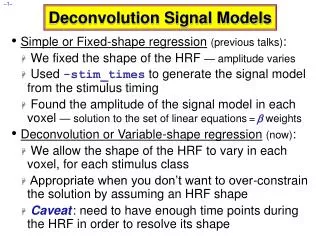
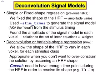
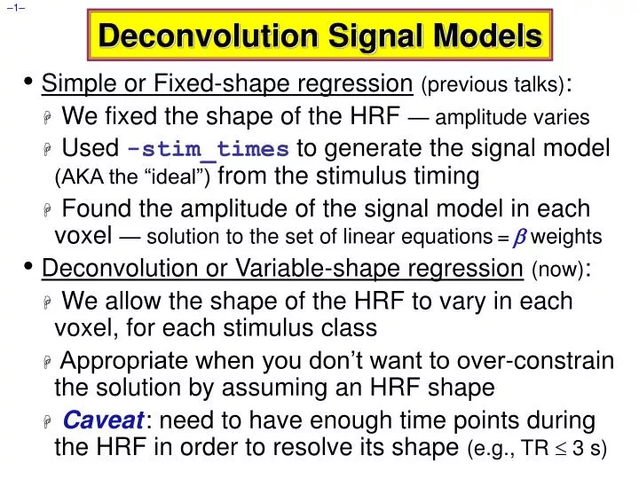
Deconvolution Signal Models. Simple or Fixed-shape regression (previous talks) : We fixed the shape of the HRF — amplitude varies Used -stim_times to generate the signal model (AKA the “ideal”) from the stimulus timing

E N D
Deconvolution Signal Models • Simple or Fixed-shape regression(previous talks): • We fixed the shape of the HRF — amplitude varies • Used -stim_times to generate the signal model (AKA the “ideal”) from the stimulus timing • Found the amplitude of the signal model in each voxel — solution to the set of linear equations= weights • Deconvolution or Variable-shape regression(now): • We allow the shape of the HRF to vary in each voxel, for each stimulus class • Appropriate when you don’t want to over-constrain the solution by assuming an HRF shape • Caveat: need to have enough time points during the HRF in order to resolve its shape (e.g., TR 3 s)
Deconvolution: Pros & Cons (+ & –) • Letting HRF shape varies allows for subject and regional variability in hemodynamics • Can test HRF estimate for different shapes (e.g., are later time points more “active” than earlier?) • Need to estimate more parameters for each stimulus class than a fixed-shape model (e.g., 4-15 vs. 1 parameter=amplitude of HRF) • Which means you need more data to get the same statistical power (assuming that the fixed-shape model you would otherwise use was in fact “correct”) • Freedom to get any shape in HRF results can give weird shapes that are difficult to interpret
Expressing HRF via Regression Unknowns • The tool for expressing an unknown function as a finite set of numbers that can be fit via linear regression is an expansion in basis functions • The basis functions q(t) & expansion order p are known • Larger p more complex shapes & more parameters • The unknowns to be found (in each voxel) comprises the set of weightsqfor each q(t) • weights appear only by multiplying known values, and HRF only appears in signal model by linear convolution (addition) with known stimulus timing • Resulting signal model still solvable by linear regression
3dDeconvolve with “Tent Functions” • Need to describe HRF shape and magnitude with a finite number of parameters • And allow for calculation of h(t) at any arbitrary point in time after the stimulus times: • Simplest set of such functions are tent functions • Also known as “piecewise linear splines” h N.B.: cubic splines are also available time t=0 t=TR t=2TR t=3TR t=4TR t=5TR
A Tent Functions = Linear Interpolation • Expansion of HRF in a set of spaced-apart tent functions is the same as linear interpolation between “knots” • Tent function parameters are also easily interpreted as function values (e.g., 2 = response at time t = 2L after stim) • User must decide on relationship of tent function grid spacing L and time grid spacing TR (usually would choose L TR) • In 3dDeconvolve: specify duration of HRF and number of parameters (details shown a few slides ahead) h 2 3 N.B.: 5 intervals = 6 weights 1 4 0 5 time “knot” times 0 L 2L 3L 4L 5L
Tent Functions: Average Signal Change • For input to group analysis, usually want to compute average signal change • Over entire duration of HRF (usual) • Over a sub-interval of the HRF duration (sometimes) • In previous slide, with 6 weights, average signal change is 1/2 0 +1 +2 +3 +4 +1/2 5 • First and last weights are scaled by half since they only affect half as much of the duration of the response • In practice, may want to use 00 since immediate post-stimulus response is not neuro-hemodynamically relevant • All weights (for each stimulus class) are output into the “bucket” dataset produced by 3dDeconvolve • Can then be combined into a single number using 3dcalc
0 +4 0 +4 0 +4 1 +5 1 +5 1 +5 3 3 3 2 2 2 Equations at each data time point: Cannot tell 0 from 4, or 1 from 5 0 1 2 3 HRF from stim #1 0 0 0 1 1 1 2 2 2 3 3 3 4 4 4 5 5 5 A stim #1 Deconvolution and Collinearity • Regular stimulus timing can lead to collinearity! time Tail of HRF from #1 overlaps head of HRF from #2, etc
Deconvolution Example - The Data • cd AFNI_data2 • data is in ED/ subdirectory (10 runs of 136 images each; TR=2 s) • script = s1.afni_proc_command(in AFNI_data2/ directory) • stimuli timing and GLT contrast files in misc_files/ • this script runs program afni_proc.py to generate a shell script with all AFNI commands for single-subject analysis • Run by typing tcsh s1.afni_proc_command; then copy/paste tcsh -x proc.ED.8.glt |& tee output.proc.ED.8.glt • Event-related study from Mike Beauchamp • 10 runs with four classes of stimuli (short videos) • Tools moving (e.g., a hammer pounding) - ToolMovie • People moving (e.g., jumping jacks) - HumanMovie • Points outlining tools moving (no objects, just points) - ToolPoint • Points outlining people moving - HumanPoint • Goal: find brain area that distinguishes natural motions (HumanMovie and HumanPoint) from simpler rigid motions (ToolMovie and ToolPoint) Text output from programs goes to screen andfile
Master Script for Data Analysis • Master script program • 10 input datasets • Set output filenames • Copy anat to output dir • Discard first 2 TRs • Where to align all EPIs • Stimulus timing files (4) • Stimulus labels • HRF model • Specifies that next lines are options to be passed to 3dDeconvolve directly (in this case, the GLTs we want computed) afni_proc.py \ -dsets ED/ED_r??+orig.HEAD \ -subj_id ED.8.glt \ -copy_anat ED/EDspgr \ -tcat_remove_first_trs 2 \ -volreg_align_to first \ -regress_stim_times misc_files/stim_times.*.1D \ -regress_stim_labels ToolMovie HumanMovie \ ToolPoint HumanPoint \ -regress_basis 'TENT(0,14,8)' \ -regress_opts_3dD \ -gltsym ../misc_files/glt1.txt -glt_label 1 FullF \ -gltsym ../misc_files/glt2.txt -glt_label 2 HvsT \ -gltsym ../misc_files/glt3.txt -glt_label 3 MvsP \ -gltsym ../misc_files/glt4.txt -glt_label 4 HMvsHP \ -gltsym ../misc_files/glt5.txt -glt_label 5 TMvsTP \ -gltsym ../misc_files/glt6.txt -glt_label 6 HPvsTP \ -gltsym ../misc_files/glt7.txt -glt_label 7 HMvsTM } This script generates file proc.ED.8.glt(180 lines), which contains all the AFNI commands to produce analysis results into directory ED.8.glt.results/ (148 files)
Shell Script for Deconvolution - Outline • Copy datasets into output directory for processing • Examine each imaging run for outliers: 3dToutcount • Time shift each run’s slices to a common origin: 3dTshift • Registration of each imaging run: 3dvolreg • Smooth each volume in space (136 sub-bricks per run): 3dmerge • Create a brain mask: 3dAutomask and 3dcalc • Rescale each voxel time series in each imaging run so that its average through time is 100: 3dTstat and 3dcalc • If baseline is 100, then a q of 5 (say) indicates a 5% signal change in that voxel at tent function knot #q after stimulus • Biophysics: believe % signal change is relevant physiological parameter • Catenate all imaging runs together into one big dataset (1360 time points): 3dTcat • This dataset is useful for plotting -fitts output from 3dDeconvolve and visually examining time series fitting • Compute HRFs and statistics: 3dDeconvolve
Script - 3dToutcount # set list of runs set runs = (`count -digits 2 1 10`) # run 3dToutcount for each run foreach run ( $runs ) 3dToutcount -automask pb00.$subj.r$run.tcat+orig > outcount_r$run.1D end Via 1dplot outcount_r??.1D 3dToutcount searches for “outliers” in data time series; You should examine noticeable runs & time points
Script - 3dTshift # run 3dTshift for each run foreach run ( $runs ) 3dTshift -tzero 0 -quintic -prefix pb01.$subj.r$run.tshift \ pb00.$subj.r$run.tcat+orig end • Produces new datasets where each time series has been shifted to have the same time origin • -tzero 0 means that all data time series are interpolated to match the time offset of the first slice • Which is what the slice timing files usually refer to • Quintic (5th order) polynomial interpolation is used • 3dDeconvolve will be run on these time-shifted datasets • This is mostly important for Event-Related FMRI studies, where the response to the stimulus is briefer than for Block designs • (Because the stimulus is briefer) • Being a little off in the stimulus timing in a Block design is not likely to matter much
Script - 3dvolreg # align each dset to the base volume foreach run ( $runs ) 3dvolreg -verbose -zpad 1 -base pb01.$subj.r01.tshift+orig'[0]' \ -1Dfile dfile.r$run.1D -prefix pb02.$subj.r$run.volreg \ pb01.$subj.r$run.tshift+orig end • Produces new datasets where each volume (one time point) has been aligned (registered) to the #0 time point in the #1 dataset • Movement parameters are saved into files dfile.r$run.1D • Will be used as extra regressors in 3dDeconvolveto reduce motion artifacts • 1dplot -volreg dfile.rall.1D • Shows movement parameters for all runs (1360 time points) in degrees and millimeters • Very important to look at this graph! • Excessive movement can make an imaging run useless — 3dvolreg won’t be able to compensate • Pay attention to scale of movements: more than about 2 voxel sizes in a short time interval is usually bad
Script - 3dmerge # blur each volume foreach run ( $runs ) 3dmerge -1blur_fwhm 4 -doall -prefix pb03.$subj.r$run.blur \ pb02.$subj.r$run.volreg+orig end • Why Blur? Reduce noise by averaging neighboring voxels time series • White curve = Data: unsmoothed • Yellow curve = Model fit (R2=0.50) • Green curve = Stimulus timing This is an extremely good fit for ER FMRI data!
Why Blur? - 2 • fMRI activations are (usually) blob-ish (several voxels across) • Averaging neighbors will also reduce the fiendish multiple comparisons problem • Number of independent “resels” will be smaller than number of voxels (e.g., 2000 vs. 20000) • Why not just acquire at lower resolution? • To avoid averaging across brain/non-brain interfaces • To project onto surface models • Amount to blur is specified as FWHM (Full Width at Half Maximum) of spatial averaging filter (4 mm in script)
Script - 3dAutomask # create 'full_mask' dataset (union mask) foreach run ( $runs ) 3dAutomask -dilate 1 -prefix rm.mask_r$run pb03.$subj.r$run.blur+orig end # get mean and compare it to 0 for taking 'union' 3dMean -datum short -prefix rm.mean rm.mask*.HEAD 3dcalc -a rm.mean+orig -expr 'ispositive(a-0)' -prefix full_mask.$subj • 3dAutomask creates a mask of contiguous high-intensity voxels (with some hole-filling) from each imaging run separately • 3dMean and 3dcalc are used to create a mask that is the union of all the individual run masks • 3dDeconvolve analysis will be limited to voxels in this mask • Will run faster, since less data to process Automask from EPI shown in red
Script - Scaling # scale each voxel time series to have a mean of 100 # (subject to maximum value of 200) foreach run ( $runs ) 3dTstat -prefix rm.mean_r$run pb03.$subj.r$run.blur+orig 3dcalc -a pb03.$subj.r$run.blur+orig -b rm.mean_r$run+orig \ -c full_mask.$subj+orig \ -expr 'c * min(200, a/b*100)' -prefix pb04.$subj.r$run.scale end • 3dTstat calculates the mean (through time) of each voxel’s time series data • For voxels in the mask, each data point is scaled (multiplied) using 3dcalc so that it’s time series will have mean=100 • If an HRF regressor has max amplitude=1, then its coefficient will represent the percent signal change (from the mean) due to that part of the signal model • Scaled images are very boring to view • No spatial contrast by design! • Graphs have common baseline now
Script - 3dDeconvolve } 3dDeconvolve -input pb04.$subj.r??.scale+orig.HEAD -polort 2 \ -mask full_mask.$subj+orig -basis_normall 1 -num_stimts 10 \ -stim_times 1 stimuli/stim_times.01.1D 'TENT(0,14,8)' \ -stim_label 1 ToolMovie \ -stim_times 2 stimuli/stim_times.02.1D 'TENT(0,14,8)' \ -stim_label 2 HumanMovie \ -stim_times 3 stimuli/stim_times.03.1D 'TENT(0,14,8)' \ -stim_label 3 ToolPoint \ -stim_times 4 stimuli/stim_times.04.1D 'TENT(0,14,8)' \ -stim_label 4 HumanPoint \ -stim_file 5 dfile.rall.1D'[0]' -stim_base 5 -stim_label 5 roll \ -stim_file 6 dfile.rall.1D'[1]' -stim_base 6 -stim_label 6 pitch \ -stim_file 7 dfile.rall.1D'[2]' -stim_base 7 -stim_label 7 yaw \ -stim_file 8 dfile.rall.1D'[3]' -stim_base 8 -stim_label 8 dS \ -stim_file 9 dfile.rall.1D'[4]' -stim_base 9 -stim_label 9 dL \ -stim_file 10 dfile.rall.1D'[5]' -stim_base 10 -stim_label 10 dP \ -iresp 1 iresp_ToolMovie.$subj -iresp 2 iresp_HumanMovie.$subj \ -iresp 3 iresp_ToolPoint.$subj -iresp 4 iresp_HumanPoint.$subj \ -gltsym ../misc_files/glt1.txt -glt_label 1 FullF \ -gltsym ../misc_files/glt2.txt -glt_label 2 HvsT \ -gltsym ../misc_files/glt3.txt -glt_label 3 MvsP \ -gltsym ../misc_files/glt4.txt -glt_label 4 HMvsHP \ -gltsym ../misc_files/glt5.txt -glt_label 5 TMvsTP \ -gltsym ../misc_files/glt6.txt -glt_label 6 HPvsTP \ -gltsym ../misc_files/glt7.txt -glt_label 7 HMvsTM \ -fout -tout -full_first -x1D Xmat.x1D -fitts fitts.$subj -bucket stats.$subj 4 stim types } motion params } HRF outputs } GLTs
Results: Humans vs. Tools • Color overlay: HvsT GLT contrast • Blue(upper) graphs: Human HRFs • Red(lower) graphs: Tool HRFs
Script - X Matrix Via 1grayplot -sep Xmat.x1D
Script - Random Comments • -polort 2 • Sets baseline (detrending) to use quadratic polynomials—in each run • -mask full_mask.$subj+orig • Process only the voxels that are nonzero in this mask dataset • -basis_normall 1 • Make sure that the basis functions used in the HRF expansion all have maximum magnitude=1 • -stim_times 1 stimuli/stim_times.01.1D 'TENT(0,14,8)' -stim_label 1 ToolMovie • The HRF model for the ToolMovie stimuli starts at 0 s after each stimulus, lasts for 14 s, and has 8 basis tent functions • Which have knots (breakpoints) spaced 14/(8-1)=2 s apart • -iresp 1 iresp_ToolMovie.$subj • The HRF model for the ToolMovie stimuli is output into dataset iresp_ToolMovie.ED.8.glt+orig
Script - GLTs • -gltsym ../misc_files/glt2.txt -glt_label 2 HvsT • File ../misc_files/glt2.txt contains 1 line of text: • -ToolMovie +HumanMovie -ToolPoint +HumanPoint • This is the “Humans vs. Tools” HvsT contrast shown on Results slide • This GLT means to take all 8 coefficients for each stimulus class and combine them with additions and subtractions as ordered: • This test is looking at the integrated (summed) response to the “Human” stimuli and subtracting it from the integrated response to the “Tool” stimuli • Combining subsets of the weights is also possible with -gltsym: • +HumanMovie[2..6] -HumanPoint[2..6] • This GLT would add up just the #2,3,4,5, & 6 weights for one type of stimulus and subtract the sum of the #2,3,4,5, & 6 weights for another type of stimulus • And also produce F- and t-statistics for this linear combination
+ToolMovie +HumanMovie +ToolPoint +HumanPoint 4 rows Script - Multi-Row GLTs • GLTs presented up to now have had one row • Testing if some linear combination of weights is nonzero; test statistic is t or F (F=t2 when testing a single number) • Testing if the X matrix columns, when added together to form one column as specified by the GLT (+ and –), explain a significant fraction of the data time series (equivalent to above) • Can also do a single test to see if several different combinations of weights are all zero -gltsym ../misc_files/glt1.txt -glt_label 1 FullF • Tests if any of the stimulus classes have nonzero integrated HRF (each name means “add up those weights”) : DOF=(4,1292) • Different than the default “Full F-stat” produced by 3dDeconvolve, which tests if any of the individual weights are nonzero: DOF=(32,1292)
Two Possible Formats for -stim_times 4.7 9.6 11.8 19.4 • If you don’t use -local_times or -global_times, 3dDeconvolve will guess which way to interpret numbers: • A single column of numbers (GLOBAL times) • One stimulus time per row • Times are relative to first image in dataset being at t=0 • May not be simplest to use if multiple runs are catenated • One row for each run within a catenated dataset (LOCAL times) • Each time in jth row is relative to start of run #j being t=0 • If some run has NO stimuli in the given class, just put a single “*” in that row as a filler • Different numbers of stimuli per run are OK • At least one row must have more than 1 time (so that the LOCAL type of timing file can be told from the GLOBAL) • Two methods are available because of users’ diverse needs • N.B.: if you chop first few images off the start of each run, the inputs to -stim_times must be adjusted accordingly! • Better to use -CENSORTR to tell 3dDeconvolve just to ignore those points 4.7 9.6 11.8 19.4 * 8.3 10.6
More information about -stim_times and its variants is in the afni07_advanced talk
Spatial Models of Activation • Smooth data in space before analysis • Average data across anatomically-selected regions of interest ROI (before or after analysis) • Labor intensive (i.e., hire more students) • Reject isolated small clusters of above-threshold voxels after analysis
Spatial Smoothing of Data • Reduces number of comparisons • Reduces noise (by averaging) • Reduces spatial resolution • Blur it enough: Can make FMRI results look like low resolution (1990s) PET data • Smart smoothing: average only over nearby brain or gray matter voxels • Uses resolution of FMRI cleverly • 3dBlurToFWHM and 3dBlurInMask • Or: average over selected ROIs • Or: cortical surface based smoothing
3dBlurToFWHM • New program to smooth FMRI time series datasets to a specified smoothness (as estimated by FWHM of noise spatial correlation function) • Don’t just add smoothness (à la 3dmerge) but control it (locally and globally) • Goal: use datasets from diverse scanners • Why blur FMRI time series? • Averaging neighbors will reduce noise • Activations are (usually) blob-ish (several voxels across) • Diminishes the multiple comparisons problem • 3dBlurToFWHM and 3dBlurInMask blur only inside a mask region • To avoid mixing air (noise-only) and brain voxels • Partial Differential Equation (PDE) based blurring method • 2D (intra-slice) or 3D blurring
Spatial Clustering • Analyze data, create statistical map (e.g., t statistic in each voxel) • Threshold map at a low tvalue, in each voxel separately • Will have many false positives • Threshold map by rejecting clusters of voxels below a given size • Can control false-positive rate by adjusting t threshold and cluster-size thresholds together
Multi-Voxel StatisticsSpatial Clustering&False Discovery Rate:“Correcting” the Significance
Basic Problem • Usually have 30–200K FMRI voxels in the brain • Have to make at least one decision about each one: • Is it “active”? • That is, does its time series match the temporal pattern of activity we expect? • Is it differentially active? • That is, is the BOLD signal change in task #1 different from task #2? • Statistical analysis is designed to control the error rate of these decisions • Making lots of decisions: hard to get perfection in statistical testing
Multiple Testing Corrections • Two types of errors • What is H0 in FMRI studies? H0: no effect (activation, difference, …) at a voxel • Type I error= Prob(reject H0 when H0is true) = false positive = p value Type II error= Prob(accept H0 when H1is true) = false negative = β power = 1–β = probability of detecting true activation • Strategy: controlling type I error while increasing power (decreasing type II errors) • Significance level (magic number 0.05) : p <
Family-Wise Error (FWE) • Multiple testing problem: voxel-wise statistical analysis • With N voxels, what is the chance to make a false positive error (Type I) in one or more voxels? Family-Wise Error: FW = 1–(1–p)N→1 as N increases • For Np small (compared to 1), FW Np • N 20,000+ voxels in the brain • To keep probability of even one false positive FW < 0.05 (the “corrected” p-value), need to have p < 0.05/2104=2.510–6 • This constraint on the per-voxel (“uncorrected”)p-value is so stringent that we’ll end up rejecting a lot of true positives (Type II errors) also, just to be safe on the Type I error rate • Multiple testing problem in FMRI • 3 occurrences of multiple tests: individual, group, and conjunction • Group analysis is the most severe situation (have the least data, considered as number of independent samples = subjects)
Two Approaches to the “Curse of Multiple Comparisons” • Control FWE to keep expected total number of false positives below 1 • Overall significance: FW = Prob(≥ one false positive voxel in the whole brain) • Bonferroni correction: FW = 1– (1–p)NNp, if p << N–1 • Use p=/N as individual voxel significance level to achieve FW = • Too stringent and overly conservative: p=10–8…10–6 • Something to rescue us from this hell of statistical super-conservatism? • Correlation: Voxels in the brain are not independent • Especially after we smooth them together! • Means that Bonferroni correction is way way too stringent • Contiguity: Structures in the brain activation map • We are looking for activated “blobs”: the chance that pure noise (H0) will give a set of seemingly-activated voxels next to each other is lower than getting false positives that are scattered around far apart • Control FWE based on spatial correlation (smoothness of image noise)and minimum cluster size we are willing to accept • Control false discovery rate (FDR) • FDR = expected proportion of false positive voxels among all detected voxels • Give up on the idea of having (almost) no false positives at all
Cluster Analysis: 3dClustSim • FWE control in AFNI • Monte Carlo simulations with program 3dClustSim • Named for a place where primary attractions are randomization experiments • Randomly generate some number (e.g., 1000) of brain volumes with white noise (spatially uncorrelated) • That is, each “brain” volume is purely in H0 = no activation • Noise images can be blurred to mimic the smoothness of real data • Count number of voxels that are false positives in each simulated volume • Including how many are false positives that are spatially together in clusters of various sizes (1, 2, 3, …) • Parameters to program • Size of dataset to simulate • Mask (e.g., to consider only brain-shaped regions in the 3D brick) • Spatial correlation FWHM: from 3dBlurToFWHM or 3dFWHMx • Connectivity radius: how to identify voxels belonging to a cluster? • Default = NN connection = touching faces • Individual voxel significance level = uncorrected p-value • Output • Simulated (estimated) overall significance level (corrected p-value) • Corresponding minimum cluster size at the input uncorrected p-value
# 3dClustSim -nxyz 64 64 30 -dxyz 3 3 3 -fwhm 7 # Grid: 64x64x30 3.00x3.00x3.00 mm^3 (122880 voxels) # CLUSTER SIZE THRESHOLD(pthr,alpha) in Voxels # -NN 1 | alpha = Prob(Cluster >= given size) # pthr | 0.100 0.050 0.020 0.010 # ------ | ------ ------ ------ ------ 0.020000 89.4 99.9 114.0 123.0 0.010000 56.1 62.1 70.5 76.6 0.005000 38.4 43.3 49.4 53.6 0.002000 25.6 28.8 33.3 37.0 0.001000 19.7 22.2 26.0 28.6 0.000500 15.5 17.6 20.5 22.9 0.000200 11.5 13.2 16.0 17.7 0.000100 9.3 10.9 13.0 14.8 • Example: 3dClustSim -nxyz 64 64 30 -dxyz 3 3 3 -fwhm 7 At a per-voxel p=0.005, a cluster should have 44+ voxels to occur with < 0.05 from noise only p-value of threshold 3dClustSim can be run by afni_proc.py and used in AFNI Clusterize GUI
–38– False Discovery Rate in • Situation: making many statistical tests at once • e.g, Image voxels in FMRI; associating genes with disease • Want to set threshold on statistic (e.g., F-or t-value) to control false positive error rate • Traditionally: set threshold to control probability of making a single false positive detection • But if we are doing 1000s (or more) of tests at once, we have to be very stringent to keep this probability low • FDR: accept the fact that there will be multiple erroneous detections when making lots of decisions • Control the fraction of positive detections that are wrong • Of course, no way to tell which individual detections are right! • Or at least: control the expected value of this fraction
–39– FDR: q • Given some collection of statistics (say, F-values from 3dDeconvolve), set a threshold h • The uncorrectedp-value of h is the probability that F > h when the null hypothesis is true (no activation) • “Uncorrected” means “per-voxel” • The “corrected” p-value is the probability that any voxel is above threshold in the case that they are all unactivated • If have N voxels to test, pcorrected = 1–(1–p)N Np (for small p) • Bonferroni: to keep pcorrected< 0.05, need p < 0.05 / N, which is very tiny • The FDR q-value of h is the fraction of false positives expected when we set the threshold to h • Smaller q is “better” (more stringent = fewer false detections)
Red = ps from Full-F (real data) Black = ps from pure noise (simulation) (baseline level=false +) True + False + threshold h Basic Ideas Behind FDR q • If all the null hypotheses are true, then the statistical distribution of the p-values will be uniform • Deviations from uniformity at low p-values true positives • Baseline of uniformity indicates how many true negatives are hidden amongst in the low p-value region 31,555 voxels 50 histogram bins
–46– FDR curves: h vs. q • 3dDeconvolve, 3dANOVAx, 3dttest, and 3dNLfim now compute FDR curves for all statistical sub-bricks and store them in output header • 3drefit -addFDR does same for other datasets • 3drefit -unFDR can be used to delete such info • AFNI now shows p-andq-values below the threshold slider bar • Interpolates FDR curve • from header (thresholdzq) • Can be used to adjust threshold by “eyeball” q = N/A means it’s not available MDF hint = “missed detection fraction”
–47– FDR Statistical Issues • FDR is conservative (q-values are too large) when voxels are positively correlated (e.g., from spatially smoothing) • Correcting for this is not so easy, since q depends on data (including true positives), so a simulation like 3dClustSim is hard to conceptualize • At present, FDR is an alternative way of controlling false positives, vs. 3dClustSim(clustering) • Thinking about how to combine FDR and clustering • Accuracy of FDR calculation depends on p-values being uniformly distributed under the null hypothesis • Statistic-to-p conversion should be accurate, which means that null F-distribution (say) should be correctly estimated • Serial correlation in FMRI time series means that 3dDeconvolve denominator DOF is too large • p-values will be too small, so q-values will be too small • 3dREMLfit can ride to the rescue!
These 2 methods control Type I error in different sense FWE: FW = Prob (≥ one false positive voxel/cluster in the whole brain) Frequentist’s perspective: Probability among many hypothetical activation maps gathered under identical conditions Advantage: can directly incorporate smoothness into estimate of FW FDR = expected fraction of false positive voxels among all detected voxels Focus: controlling false positives among detected voxels in one activation map, as given by the experiment at hand Advantage: not afraid of making a few Type I errors in a large field of true positives Concrete example Individual voxel p = 0.001 for a brain of 25,000 EPI voxels Uncorrected →25 false positive voxels in the brain FWE: corrected p = 0.05 →5% of the time would expect one or more false positive clusters in the entire volume of interest FDR: q = 0.05 →5% of voxels among those positively labeled ones are false positive What if your favorite blob fails to survive correction? Tricks (don’t tell anyone we told you about these) One-tail t-test? ROI-based statistics – e.g., grey matter mask, or whatever regions you focus on Analysis on surface; or, Use better group analysis tool (3dLME, 3dMEMA, etc.) FWE or FDR?