Download
1 / 55
600 likes | 824 Views
Imaging and Deconvolution David J. Wilner Harvard-Smithsonian CfA. Observing with ALMA: A Workshop McMaster University, June 1, 2009. References. Thompson, A.R., Moran, J.M., & Swensen, G.W. 1986, “Interferometry and Synthesis in Radio Astronomy” (New York: Wiley); 2nd edition 2001

E N D
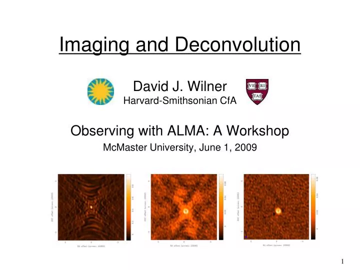
Imaging and DeconvolutionDavid J. WilnerHarvard-Smithsonian CfA Observing with ALMA: A Workshop McMaster University, June 1, 2009
References • Thompson, A.R., Moran, J.M., & Swensen, G.W. 1986, “Interferometry and Synthesis in Radio Astronomy” (New York: Wiley); 2nd edition 2001 • NRAO Summer School proceedings • http://www.aoc.nrao.edu/events/synthesis/ • Perley, R.A., Schwab, F.R. & Bridle, A.H., eds. 1989, ASP Conf. Series 6, Synthesis Imaging in Radio Astronomy (San Francisco: ASP) • Chapter 6: Imaging (Sramek & Schwab), Chapter 8: Deconvolution (Cornwell) • T. Cornwell 2002, S. Bhatnagar 2004, 2006 “Imaging and Deconvolution” • IRAM Summer School proceedings • http://www.iram.fr/IRAMFR/IS/archive.html • Guilloteau, S., ed. 2000, “IRAM Millimeter Interferometry Summer School” • Chapter 13: Imaging Principles, Chapter 16: Imaging in Practice (Guilloteau) • http://www.iram.fr/IRAMFR/IS/school.htm • J. Pety 2004 “Imaging, Deconvolution & Image Analysis” • J. Pety 2006 “Standard Imaging and Deconvolution” • J. Pety 2008 “Imaging and Deconvolution Part I” and “Part II” • CARMA Summer School proceedings • http://carma.astro.umd.edu/wiki/index.php/School2008 • M. Wright “The Complete Mel Lectures” • talks by many practitioners in the field
Visibility and Sky Brightness • from the van Citttert-Zernike theorem (TMS Appendix 3.1) • for small fields of view: the complex visibility,V(u,v) is the 2D Fourier transform of the brightness on the sky,T(x,y) • u,v (wavelengths) are spatial frequencies in E-W and N-S directions, i.e. the baseline lengths • x,y (rad) are angles in tangent plane relative to a reference position in the E-W and N-S directions y x T(x,y)
The Fourier Transform • Fourier theory states that any signal (including images) can be expressed as a sum of sinusoids • (x,y) plane and (u,v) plane are conjugate coordinates T(x,y) V(u,v) = FT{T(x,y)} • the Fourier Transform contains all information of original Jean Baptiste Joseph Fourier 1768-1830 signal 4 sinusoidsl sum
The Fourier Domain • acquire comfort with the Fourier domain… • in older texts, functions and their Fourier transforms occupy upper and lower domains, as if “functions circulated at ground level and their transforms in the underworld’’ (Bracewell 1965) • a few properties of the Fourier transform: • scaling: • shifting: • convolution/multiplication: • sampling theorem:
Some 2D Fourier Transform Pairs • Amp{V(u,v)} T(x,y) Function Constant Gaussian Gaussian narrow features transform to wide features (and vice-versa)
More 2D Fourier Transform Pairs • Amp{V(u,v)} T(x,y) Gaussian Gaussian elliptical Gaussian elliptical Gaussian orientations are orthogonal in the (x,y) and (u,v) planes
More 2D Fourier Transform Pairs • Amp{V(u,v)} T(x,y) Disk Bessel sharp edges result in many high spatial frequencies
More 2D Fourier Transform Pairs • Amp{V(u,v)} T(x,y) complicated structure on many scales
Amplitude and Phase • complex numbers: (real, imaginary) or (amplitude, phase) • amplitude tells “how much” of a certain frequency component, phase tells “where” • T(x,y) • Amp{V(u,v)} • Pha{V(u,v)}
Amplitude and Phase • complex numbers: (real, imaginary) or (amplitude, phase) • amplitude tells “how much” of a certain frequency component, phase tells “where” • T(x,y) • Amp{V(u,v)} • Pha{V(u,v)}
Two Visibilities for One Measurement • T(x,y) is real, but V(u,v) is complex (in general) • V(-u,-v) = V*(u,v) where * is complex conjugation (Hermitian) • V(u=0,v=0) integral of T(x,y)dxdy = total flux • T(x,y) • Amp{V(u,v)}
Aperture Synthesis • sample V(u,v) at enough points to synthesis the equivalent large aperture of size (umax,vmax) • 1 pair of telescopes 1 (u,v) sample at a time • N telescopes number of samples = N(N-1)/2 • reconfigure physical layout of N telescopes for more • fill in (u,v) plane by making use of Earth rotation: Sir Martin Ryle, 1974 Nobel Prize in Physics Sir Martin Ryle 1918-1984 2 configurations of 8 SMA antennas 345 GHz Dec = -24 deg
IRAM PdBI ATCA SMA Examples of Millimeter Aperture Synthesis Telescopes CARMA (=OVRO+BIMA) EVLA
Imaging: (u,v) plane Sampling • in aperture synthesis, V(u,v) samples are limited by number of telescopes, and Earth-sky geometry • high spatial frequencies • maximum angular resolution • low spatial frequencies • extended structures invisible • irregular within high/low limits • sampling theorem violated • information lost
Formal Description • sample Fourier domain at discrete points • the inverse Fourier transform is • the convolution theorem tells us where (the point spread function) Fourier transform of sampled visibilities yields the true sky brightness convolved with the point spread function (the “dirty image” is the true image convolved with the “dirty beam”)
Dirty Beam and Dirty Image b(x,y) (dirty beam) B(u,v) TD(x,y) (dirty image) T(x,y)
How to analyze interferometer data? • uv plane analysis • best for “simple” sources, e.g. point sources, disks • image plane analysis • Fourier transform V(u,v) samples to image plane, get TD(x,y) • but difficult to do science on dirty image • deconvolve b(x,y) from TD(x,y) to determine (model of) T(x,y) visibilities dirty image sky brightness Fourier transform deconvolve
Details of the Dirty Image • Fourier Transform • Fast Fourier Transform (FFT) much faster than simple Fourier summation, O(NlogN) for 2N x 2N image • FFT requires data on regularly spaced grid • aperture synthesis observations not on a regular grid… • “Gridding” is used to resample V(u,v) for FFT • customary to use a convolution technique • visibilities are noisy samples of a smooth function • nearby visibilities not independent • use special (“Spheroidal”) functions with nice properties • fall off quickly in (u,v) plane (not too much smoothing) • fall off quickly in image plane (avoid aliasing)
Primary Beam T(x,y) • A telescope does not have uniform response across the entire sky • main lobe approximately Gaussian, fwhm ~1.2/D (where D is ant diameter) = “primary beam” • limited field of view • sidelobes, error beam (sometimes important) • primary beam response modifies sky brightness: T(x,y) A(x,y)T(x,y) • correct with division by A(x,y) in image plane A(x,y) SMA 345 GHz ALMA 690 GHz T(x,y) large A(x,y) small A(x,y)
Pixel Size and Image Size • pixel size • should satisfy sampling theorem for the longest baselines, x < 1/2 umax , y < 1/2 vmax • in practice, 3 to 5 pixels across the main lobe of the dirty beam (to aid deconvolution) • e.g., SMA: 0.87mm, 500 m baselines 600 kl < 0.1 arcsec • image size • natural resolution in (u,v) plane samples FT{A(x,y)}, implies image size 2x primary beam • e.g., SMA: 0.87mm, 6 m telescope 2x 35 arcsec • if there are bright sources in the sidelobes of A(x,y), then they will be aliased into the image (need to make a larger image)
Dirty Beam Shape and Weighting • introduce weighting function W(u,v) • W modifies sidelobes of dirty beam • W is also gridded for FFT • “Natural” weighting • W(u,v) = 1/2(u,v) at points with data and zero elsewhere where 2(u,v) is the noise variance of the (u,v) sample • maximizes point source sensitivity (lowest rms in image) • gives more weight to shorter baselines (larger spatial scales), degrades resolution
Dirty Beam Shape and Weighting • “Uniform” weighting • W(u,v) is inversely proportional to local density of (u,v) points, so sum of weights in a (u,v) cell is a constant (or zero) • fills (u,v) plane more uniformly, so (outer) sidelobes are lower • gives more weight to long baselines and therefore higher angular resolution • degrades point source sensitivity (higher rms in image) • can be trouble with sparse sampling (cells with few data points have same weight as cells with many data points)
Dirty Beam Shape and Weighting • “Robust” (Briggs) weighting • variant of “uniform” that avoids giving too much weight to cell with low natural weight • implementations differ, e.g. SN is natural weight of a cell, St is a threshold • large threshold natural weighting • small threshold uniform weighting • a parameter allows continuous variation between optimal angular resolution and optimal point source sensitivity
Dirty Beam Shape and Weighting • “Tapering” • apodize the (u,v) sampling by a Gaussian t = tapering parameter (in k; arcsec) • like smoothing in the image plane (convolution by a Gaussian) • gives more weight to shorter baselines, degrades angular resolution • degrades point source sensitivity but can improve sensitivity to extended structure • could use elliptical Gaussian, other function • limits to usefulness
Weighting and Tapering: Noise Natural 0.77x0.62 =1.0 Robust 0 0.41x0.36 =1.6 Uniform 0.39x0.31 =3.7 Robust 0 + Taper 0.77x0.62 =1.7
Weighting and Tapering: Summary • imaging parameters provide a lot of freedom • appropriate choice depends on science goals
Deconvolution • difficult to do science on dirty image • deconvolve b(x,y) from TD(x,y) to recover T(x,y) • information is missing, so be careful! • there’s noise, too dirty image “CLEAN” image
Deconvolution Philosophy • to keep you awake at night • an infinite number of T(x,y) compatible with sampled V(u,v), i.e. “invisible” distributions R(x,y) where b(x,y) R(x,y) = 0 • no data beyond umax,vmax unresolved structure • no data within umin,vmin limit on largest size scale • holes between umin,vmin and umax,vmax sidelobes • noise undetected/corrupted structure in T(x,y) • no unique prescription for extracting optimum estimate of true sky brightness from visibility data • deconvolution • uses non-linear techniques effectively interpolate/extrapolate samples of V(u,v) into unsampled regions of the (u,v) plane • aims to find a sensible model of T(x,y) compatible with data • requires a priori assumptions about T(x,y)
Deconvolution Algorithms • most common algorithms in radio astronomy • CLEAN (Högbom 1974) • a priori assumption: T(x,y) is a collection of point sources • variants for computational efficiency, extended structure • Maximum Entropy (Gull and Skilling 1983) • a priori assumption: T(x,y) is smooth and positive • vast literature about the deep meaning of entropy (Bayesian) • hybrid approaches of these can be effective • deconvolution requires knowledge of beam shape and image noise properties (usually OK for aperture synthesis) • atmospheric seeing can modify effective beam shape • deconvolution process can modify image noise properties
Basic CLEAN Algorithm • Initialize • a residual map to the dirty map • a Clean component list to empty • Identify strongest feature in residual map as a point source • Add a fraction g (the loop gain) of this point source to the clean component list • Subtract the fraction g times b(x,y) from residual map • If stopping criteria not reached, goto step 2 (an iteration) • Convolve Clean component (cc) list by an estimate of the main lobe of the dirty beam (the “Clean beam”) and add residual map to make the final “restored” image b(x,y) TD(x,y)
Basic CLEAN Algorithm (cont) • stopping criteria • residual map max < multiple of rms (when noise limited) • residual map max < fraction of dirty map max (dynamic range limited) • max number of clean components reached • loop gain: • good results for g ~ 0.1 to 0.3 • lower values can work better for smoother emission, g ~ 0.05 • easy to include a priori information about where to search for clean components (“clean boxes”) • very useful but potentially dangerous! • Schwarz (1978): CLEAN is equivalent to a least squares fit of sinusoids (in the absense of noise)
CLEAN CLEAN model TD(x,y) restored image residual map
CLEAN with Box CLEAN model TD(x,y) restored image residual map
CLEAN with Poor Choice of Box CLEAN model TD(x,y) restored image residual map
CLEAN Variants • Clark CLEAN • aims at faster speed for large images • Högbom-like “minor” cycle w/ truncated dirty beam, subset of largest residuals • in “major” cycle, cc’s are FFT’d and subtracted from the FFT of the residual image from the previous “major” cycle • Cotton-Schwab CLEAN (MX) • in “major” cycle, cc’s are FFT’d and subtracted from ungridded visibilities • more accurate but slower (gridding steps repeated) • Steer, Dewdny, Ito (SDI) CLEAN • aims to supress CLEAN “stripes” in smooth, extended emission • in “minor” cycles, any point in the residual map greater than a fraction (<1) of the maximum is taken as a cc • Multi-Resolution CLEAN • aims to account for coupling between pixels by extended structure • independently CLEAN a smooth map and a difference map, fewer cc’s
“Restored” Images • CLEAN beam size: • natural choice is to fit the central peak of the dirty beam with elliptical Gaussian • unit of deconvolved map is Jy per CLEAN beam area (= intensity, can convert to brightness temperature) • minimize unit problems when adding dirty map residuals • modest super resolution often OK, but be careful • “restored” image does not fit the visibility data • photometry should be done with caution • CLEAN does not conserve flux (extrapolates) • extended structure missed, attenuated, distorted • phase errors (e.g. seeing) can spread signal around
Noise in Images • point source sensitivity: straightforward • telescope area, bandwidth, integration time, weighting • in image, modify noise by primary beam response • extended source sensitivity: problematic • not quite right to divide noise by n beams covered by source: smoothing = tapering, omitting data lower limit • always missing flux at some spatial scale • be careful with low signal-to-noise images • if position known, 3 OK for point source detection • if position unknown, then 5 required (flux biased by ~1) • if < 6, cannot measure the source size (require ~3 difference between “long” and “short” baselines) • spectral lines may have unknown position, velocity, width
Maximum Entropy Algorithm • Maximize a measure of smoothness (the entropy) subject to the constraints • M is the “default image” • fast (NlogN) non-linear optimization solver due to Cornwell and Evans (1983) • optional: convolve with Gaussian beam and add residual map to make map b(x,y) TD(x,y)
Maximum Entropy Algorithm (cont) • easy to include a priori information with default image • flat default best only if nothing known (or nothing observed!) • straightforward to generalize 2to combine different observations/telescopes and obtain optimal image • many measures of “entropy” available • replace log with cosh “emptiness” (does not enforce positivity) • less robust and harder to drive than CLEAN • works well on smooth, extended emission • trouble with point source sidelobes • no noise estimate possible from image
Maximum Entropy MAXEN model TD(x,y) restored image residual map
Imaging Results Natural Weight Beam CLEAN image
Imaging Results Uniform Weight Beam CLEAN image
Imaging Results Robust=0 Beam CLEAN image
Imaging Results Robust=0 Beam MAXEN image
Example: WSB 60 Protoplanetary Disk • tune resolution and sensitivity to suit science • e.g. Andrews, Wilner et al. 2009, ApJ, in press • SMA 870 mm images of “transitional” protoplanetary disks with resolved inner holes, note images of WSB 60 500 AU
Missing Low Spatial Frequencies (I) • Large Single Telescope • make an image by scanning across the sky • all Fourier components from 0 to D sampled, where D is the telescope diameter (weighting depends on illumination) • Fourier transform single dish map = T(x,y) A(x,y), then divide by a(x,y) = FT{A(x,y)}, to estimate V(u,v) • choose D large enough to overlap interferometer samples of V(u,v) and avoid using data where a(x,y) becomes small density of uv points (u,v)
Missing Low Spatial Frequencies (II) • separate array of smaller telescopes • use smaller telescopes observe short baselines not accessible to larger telescopes • shortest baselines from larger telescopes total power maps ALMA with ACA 64 x 12 m: 12 to 14000 m +12 x 7 m: fills ~7 to 12 m + 4 x 12 m: fills 0 to ~7 m