Download
1 / 25
260 likes | 269 Views
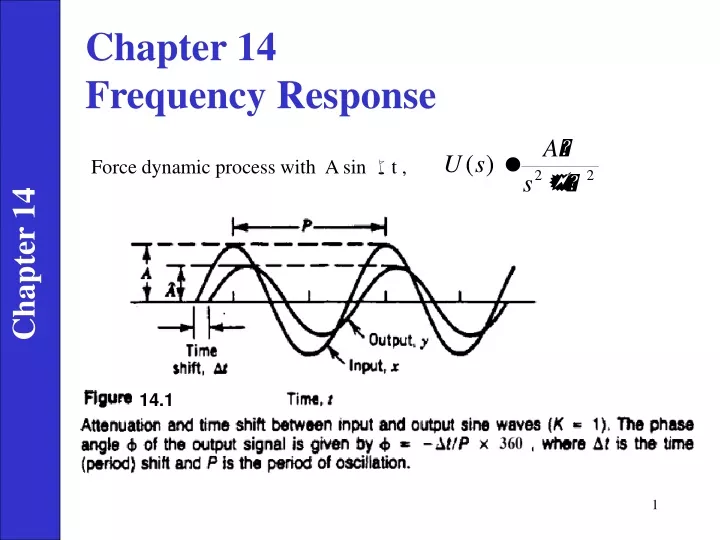
Chapter 14 Frequency Response. Force dynamic process with A sin t ,. Chapter 14. 14.1. Input: Output: is the normalized amplitude ratio ( AR ) is the phase angle, response angle ( RA ) AR and are functions of ω Assume G(s) known and let. Chapter 14.

E N D
Chapter 14 Frequency Response Force dynamic process with A sin t , Chapter 14 14.1
Input: Output: is the normalized amplitude ratio (AR) is the phase angle, response angle (RA) AR and are functions of ω Assume G(s) known and let Chapter 14
Example 14.1: Chapter 14 K1 K2
Use a Bode plot to illustrate frequency response (plot of log |G| vs. log and vs. log ) log coordinates: Chapter 14
Chapter 14 Figure 14.4 Bode diagram for a time delay, e-qs.
Example 14.3 Chapter 14
F.R. Characteristics of Controllers Recall that the F.R. is characterized by: 1. Amplitude Ratio (AR) 2. Phase Angle () For any T.F., G(s) A) Proportional Controller Chapter 14 B) PI Controller For The Bode plot for a PI controller is shown in next slide. Note b = 1/I . Asymptotic slope ( 0) is -1 on log-log plot.
Ideal PID Controller. Series PID Controller. The simplest version of the series PID controller is Chapter 14 Series PID Controller with a Derivative Filter. The series controller with a derivative filter was described in Chapter 8
Figure 14.6 Bode plots of ideal parallel PID controller and series PID controller with derivative filter (α = 1). Ideal parallel: Series with Derivative Filter: Chapter 14
Advantages of FR Analysis for Controller Design: 1. Applicable to dynamic model of any order (including non-polynomials). 2. Designer can specify desired closed-loop response characteristics. 3. Information on stability and sensitivity/robustness is provided. Disadvantage: The approach tends to be iterative and hence time-consuming -- interactive computer graphics desirable (MATLAB) Chapter 14
Controller Design by Frequency Response - Stability Margins • Analyze GOL(s) = GCGVGPGM(open loop gain) • Three methods in use: • (1) Bode plot |G|, vs. (open loop F.R.) - Chapter 14 • Nyquist plot - polar plot of G(j) - Appendix J • Nichols chart |G|, vs. G/(1+G) (closed loop F.R.) - Appendix J • Advantages: • do not need to compute roots of characteristic equation • can be applied to time delay systems • can identify stability margin, i.e., how close you are to instability. Chapter 14
Chapter 14 14.8
Frequency Response Stability Criteria • Two principal results: • 1. Bode Stability Criterion • 2. Nyquist Stability Criterion • I) Bode stability criterion • A closed-loop system is unstable if the FR of the • open-loop T.F. GOL=GCGPGVGM, has an amplitude ratio • greater than one at the critical frequency, . Otherwise • the closed-loop system is stable. • Note: where the open-loop phase angle • is -1800. Thus, • The Bode Stability Criterion provides info on closed-loop stability from open-loop FR info. • Physical Analogy: Pushing a child on a swing or bouncing a ball. Chapter 14
Example 1: A process has a T.F., And GV = 0.1, GM = 10 . If proportional control is used, determine closed-loop stability for 3 values of Kc: 1, 4, and 20. Solution: Chapter 14 The OLTF is GOL=GCGPGVGM or... The Bode plots for the 3 values of Kc shown in Fig. 14.9. Note: the phase angle curves are identical. From the Bode diagram:
Chapter 14 Figure 14.9 Bode plots for GOL = 2Kc/(0.5s + 1)3.
For proportional-only control, the ultimate gain Kcu is defined to be the largest value of Kc that results in a stable closed-loop system. • For proportional-only control, GOL= KcG and G = GvGpGm. AROL(ω)=Kc ARG(ω) (14-58) • where ARG denotes the amplitude ratio of G. • At the stability limit, ω= ωc, AROL(ωc) = 1 and Kc= Kcu. Chapter 14
Example 14.7: Determine the closed-loop stability of the system, Where GV = 2.0, GM = 0.25 and GC =KC . Find C from the Bode Diagram. What is the maximum value of Kc for a stable system? Chapter 14 Solution: The Bode plot for Kc= 1 is shown in Fig. 14.11. Note that:
Chapter 14 14.11
Ultimate Gain and Ultimate Period • Ultimate Gain: KCU = maximum value of |KC| that results in a • stable closed-loop system when proportional-only • control is used. • Ultimate Period: • KCU can be determined from the OLFR when • proportional-only control is used with KC=1. Thus • Note: First and second-order systems (without time delays) • do not have a KCU value if the PID controller action is correct. Chapter 14
Gain and Phase Margins • The gain margin (GM) and phase margin (PM) provide • measures of how close a system is to a stability limit. • Gain Margin: • Let AC = AROL at = C. Then the gain margin is • defined as: GM = 1/AC • According to the Bode Stability Criterion, GM >1 stability • Phase Margin: • Let g = frequency at which AROL = 1.0 and the • corresponding phase angle is g . The phase margin • is defined as: PM = 180° + g • According to the Bode Stability Criterion, PM >0 stability • See Figure 14.12. Chapter 14
Rules of Thumb: • A well-designed FB control system will have: • Closed-Loop FR Characteristics: • An analysis of CLFR provides useful information about control system performance and robustness. Typical desired CLFR for disturbance and setpoint changes and the corresponding step response are shown in Appendix J. Chapter 14
Chapter 14 Previous chapter Next chapter