Download
1 / 21
370 likes | 725 Views
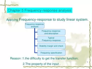
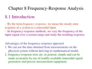
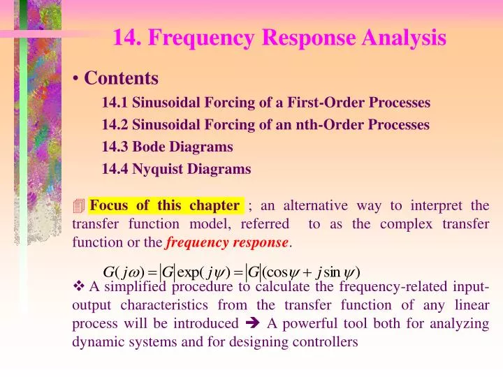
Focus of this chapter ; an alternative way to interpret the transfer function model, referred to as the complex transfer function or the frequency response .

E N D
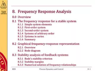
Focus of this chapter ; an alternative way to interpret the transfer function model, referred to as the complex transfer function or the frequency response. • A simplified procedure to calculate the frequency-related input-output characteristics from the transfer function of any linear process will be introduced A powerful tool both for analyzing dynamic systems and for designing controllers 14. Frequency Response Analysis • Contents 14.1 Sinusoidal Forcing of a First-Order Processes 14.2 Sinusoidal Forcing of an nth-Order Processes 14.3 Bode Diagrams 14.4 Nyquist Diagrams
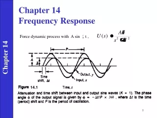
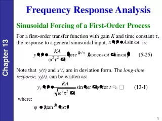
First-order process. The output response to a general sinusoidal input, is If the sine wave is continued for a long time, the exponential term becomes negligible. • Long time response or Frequency response : where . 14.1 Sinusoidal Forcing of a First-Order Processes
Figure 14.1. Attenuation and time shift between input and output sine waves( ). • Two distinctive features 1. The output sine wave has the same frequency but its phase is shifted relative to the input sine wave by the angle (referred to as the phase shift or the phase angle) ; the amount of phase shift depends on the forcing frequency. 2. The output sine wave has an amplitude that also is a function of the forcing frequency.
Amplitude ratio AR ; • Normalized amplitude ratio ARN; • Phase shift( or angle); • For a fast oscillatory input: - high frequency input ; the input signal is almost completely attenuated. • For a slowly varying input: - low frequency input ; the phase shift is very small.
For of high order stable system and sine wave input • Stable parts decayed out( as after inverse Laplace Transform). • Following term is left only. 14.2 Sinusoidal Forcing of an nth-Order Processes • This section develops a general approach for deriving the frequency response of any stable transfer function. • Partial fraction form ; (14.1)
and can be obtain by Heaviside expansion. where and . • Polar form of the complex function ; where and are the magnitude and angle of in the complex plane. Then Long-time response of (14.1) is ;
Shortcut Method for Finding Frequency Response Step 1. Set in to obtain . Step 2. Rationalize :Express as , where and are functions of and possibly model parameters, using complex conjugate multiplication. Step 3. The output sine wave has amplitude and phase angle . The amplitude ratio is and it is independent of the value of . • An unstable process does not have a “frequency response” because a sinusoidal input produces an unstable output response.
The Bode diagram consist of (1) a log-log plot of versus , and (2) a semilog plot of versus . • Process • Frequency response 14.3 Bode Diagrams • Useful for rapid analysis of the response characteristic and stability. 14.3.1 First-order system
Note) • slope of asymptote is -1 • Properties • At low frequency, as • At high frequency, as • Break frequency ( or corner) Figure 14.2. Bode diagram for a first-order process.
Step 1. Locate the break frequency . at this point is 0.707 . Step 2. Draw a horizontal asymptote( ) for low-frequency region, . Step 3. Draw the high-frequency asymptote with slope -1, intersecting with at . Step 4. Sketch the actual frequency response, using the shape shown in Figure 14.2. Step 5. At , . Locate this point and draw horizontal asymptotes at and . Sketch the phase angle curve using Figure 14.2 as a pattern or employing the data points from Table 14.1. Table14.1. Phase Angles as a Function of , First-order System • Procedure for constructing Bode diagram of first-order system.
Process • Frequency response • At low frequency, as • At high frequency, as Note) • slope of asymptote is -2 14.3.2 Second-order system Figure 14.3. Bode diagram for critically damped and overdamped second-order processes
For overdamped systems, the normalized amplitude ratio attenuated( ) for all . • For underdamped systems, the amplitude ratio plot exhibits a maximum( ) at the resonant frequency. To exist , • Feedback controllers are tuned to give a slight amount of resonant so as to speed up the controlled system response. Figure 14.4. Bode diagram for underdamped second-order processes
Step 1. Draw the low-frequency asymptote at . Step 2. At ( is the larger time constant) the slope of the asymptote changes to -1. Step 3. At the slope of the asymptote changes to -2. Step 4. Calculate several points on the actual curve and sketch it using the asymptotic representations as guidelines. • Procedure for constructing AR plot of overdamped second-order system. • Procedure for constructing AR plot of underdamped second-order system. Step 1. Draw the low-frequency asymptote at . Step 2. At the slope of the asymptote changes to -2. Step 4. Calculate several points on the actual curve and sketch it using the asymptotic representations as guidelines. The maximum value in AR will be observed only if .
; positive phase angle between and . at high frequency • The output signal amplitude becomes very large at high frequencies ( as ), a physical impossibility. 14.3.3 Process Zeros • LHP zero(= process lead) • RHP zero(= process lag) ; negative phase angle. • Nonminimum phase system; process that contain a RHP zero or time delay they exhibit more phase lag than another transfer function which has same AR plot.
1) the high frequency asymptotic slope of the AR curve is given by or 2) the phase angle for high frequency is given by where and represent the number of right-half plane and left-half plane zeros, respectively. • General rules
14.3.4 Time Delay • Frequency response • Unbounded phase lag is an important feature of a time delay. Figure 14.5. Bode diagram for a time delay.
Padé approximation • 1/1 approximation In this range, approximation gives accurate results. • 2/2 approximation Figure 14.6. Phase angle plots for time delay and for 1/1 and 2/2 Padé approximations.
14.3.5 Pure integrator 14.3.6 Pure differenciator
The Bode diagram is polar plot of depending on . 14.4 Nyquist Diagrams • Disadvantages 1. The frequency is not plotted explicitly on the abscissa. 2. It is more difficult to construct from individual transfer function than Bode diagram. • Advantages It is more compact and is sufficient for many important analytical techniques, for example, determining system stability.
Example) • Process • Frequency response Figure 14.7. The Nyquist diagram for Example. • Qualitative guidelines 1. No time delay and denominator order four or less; the Nyquist diagram terminates at the origin without encircling the origin. The point of termination will depend on numerator and denominator orders, but the total angle will be greater in absolute value than 360o. 2. Time delay with poles and zeros ; there will be infinite number of encirclement occurs if the Nyquist plot completely encloses the origin.