Download
1 / 35
380 likes | 690 Views
Migration Velocity Analysis. 01. Outline. Motivation. Estimate a more accurate velocity model for migration. Theory. Tomographic migration velocity analysis. Numerical Results. Conclusions. 02. Motivation. Forward modeling. d = L m. Kirchhoff Migration. m mig = L T d.

E N D
Outline • Motivation • Estimate a more accurate velocity model for migration • Theory • Tomographic migration velocity analysis • Numerical Results • Conclusions 02
Motivation Forward modeling d = L m Kirchhoff Migration mmig = LT d Function of velocity: LT (s) Inaccurate velocity model mmig = LTd 03
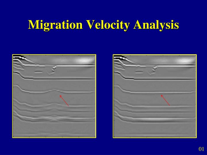
Motivation Inaccurate velocity model True velocity model True velocity model Inaccurate velocity model Goal of MVA: To get a more accurate velocity model Kirchhoff Migration Image Kirchhoff Migration Image Position error Structure error 04
Outline • Motivation • Estimate a more accurate velocity model for migration • Theory • Tomographic Migration Velocity Analysis • Numerical Results • Conclusions 05
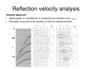
Theory The fundamental principle underlying MVA is that the migration image of the same reflector should be the same for different source, when using the correct velocity, so pre-stack common image gather (CIG) provides the information of whether the migration velocity is correct and how far away it is from the true velocity. 06
CSG #2 Theory Common Image Gather ( CIG) different CSGs CSG #1 CSG #3 Point scatterer 07
x Theory x0 Common Image Gather ( CIG) Prestack migration x0 x z s KM of CSG #3 x x0 z KM of CSG #2 z CIG KM of CSG #1 08
Theory Tomographic MVA x x0 x0 x x x0 z z z CIG s x x0 Correct Velocity z z 2000 m/s Flat 09
Theory Tomographic MVA x x0 x0 x x x0 z z z CIG s x x0 Incorrect Velocity z z 1500 m/s Curved 10
Theory Tomographic MVA CIG CIG x0 h 0 0 Z0 Zh Z (km) Z (km) 1.5 1.5 -1 Offset (km) 1 -1 Offset (km) 1 Hyperbolic approximation Zh2 = Z02 + A h2 Z0 h Zh picking depth, zero-offset depth, offset, ΔZ = Zh - Zref Zref Depth residual reference depth Usually choose Z0 as Zref 11
Theory Tomographic MVA Convert depth residual to time residual x0 xg xs Find the source-receiver pair by ray tracing to obey Snell’s law θ1 θ2 x0 xg xs t’ = LSR’ s + LRG s R’ reflector with picked depth Zh t = LSR s + LRG s R reflector with reference depth Zref Δt = t’ - t 12
Theory Tomographic MVA Update the slowness t = L s t s L raypath operator, traveltime, background slowness. Δs For a small slowness perturbation Δt = t’-t0 = LΔs = L(s’-s0) Parameterize the model as a grid of cells n Δti = Σ Δsj Δlij j=1 Δti Δsj j i traveltime residual for the raypath , slowness purturbation in grid cell Δsj Δti Back project along the raypaths to get Update the slowness with a steepest descent method sj(k+1) = sj(k+1) – α Δsj(k+1) 13
Theory Tomographic MVA n m Misfit function (k) (k) Fmisfit = Σ Σ (Δzij )2 j=1 i=1 Δzij (k) j i k picked depth residual for offset in CIG of the iteration Iteration will stop when all curved events in CIG are flatten. 14
Theory Work Flow: Observed data Migration velocity model s0 Migration velocity model sk Predict travel time by eikonal solver Pre-stack KM , form CIGs All events are flattened? Pick the depth residual automatically N Y Pick the reference depth residual (usually zero-offset) MVA finished ! Find ray paths connecting the reflector to both S and R positions Convert depth residual to travel time residual Update velocity model by back projecting the traveltime residuals along the raypaths. 15
Outline • Motivation • Estimate a more accurate velocity model for migration • Theory • Tomographic migration velocity analysis • Numerical Results • Conclusions 16
Numerical Results 2D Synthetic Model True velocity model KM image CIG H. Sun. 1999 17
Numerical Results 2D Synthetic Model KM image Homogeneous velocity model CIG H. Sun. 1999 18
Numerical Results 2D Synthetic Model KM image Final updated velocity model CIG H. Sun. 1999 19
Initial Migration Velocity Horizontal Distance (km) 0 18 0 2.1 Depth (km) (km /s) 1.5 1.5
KM Image with Initial Velocity 0 18 km 0 Depth (km) 1.5 KMVA Velocity Changes in the 1st Iteration 0 50 Depth (km) (m /s) 0 1.5
KM Image with Initial Velocity 2 km 9 km 1070 Depth (m) 1260 KM Image with Updated Velocity 1070 Depth (m) 1260
KMVA CIGs with Initial Velocity KMVA CIGs with Updated Velocity 0 Depth (km) 1.5
KMVA Velocity Changes in the 1st Iteration (CPU=6) 0 18 km 0 50 Depth (km) (m /s) 0 1.5 WMVA Velocity Changes in the 1st Iteration (CPU=1) 0 50 Depth (km) (m /s) 0 1.5
WM Image with Initial Velocity 2 km 9 km 1070 Depth (m) 1260 WM Image with Updated Velocity 1070 Depth (m) 1260
WMVA CIGs with Initial Velocity WMVA CIGs with Updated Velocity 0 Depth (km) 1.5
KM Image with Initial Velocity 2 km 9 km 1070 Depth (m) 1260 KM Image with KMVA Updated Velocity 1070 Depth (m) 1260 KM Image with WMVA Updated Velocity 1070 Depth (m) 1260
Outline • Motivation • Estimate a more accurate velocity model for migration • Theory • Tomographic migration velocity analysis • Numerical Results • Conclusions 26
Conclusions • Pre-stack migration with inaccurate velocity can bring curved events in CIGs, which provides the opportunity for migration velocity analysis. • Iterative tomographic MVA can estimate better migration velocity and improve the migration image. • Question: what are the advantages and disadvantages of migration velocity analysis compared to velocity estimation in data domain ? 27
Numerical Results 2D Field Data Initial migration velocity from NMO 0 2.1 (km /s) Depth (km) 1.5 1.5 0 18 Horizontal distance (km) H. Sun. 1999 20
Numerical Results 2D Field Data KM image with the initial velocity 0 Depth (km) 1.5 0 18 Horizontal distance (km) H. Sun. 1999 21
Numerical Results 2D Field Data KM CIGs with the initial velocity 0 Depth (km) 1.2 1.5 H. Sun. 1999 22
18 km Numerical Results KM Image with Initial Velocity 0 Depth (km) 1.5 18 0 KM Image with Updated Velocity 0 Depth (km) 23 1.5
Numerical Results KM Image with Initial Velocity 2 km 9 km 1070 Depth (m) 1260 KM Image with Updated Velocity 1070 Depth (m) 1260 24
Numerical Results KMVA CIGs with Initial Velocity KMVA CIGs with Updated Velocity 0 Depth (km) 1.5 25