Download
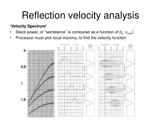
1 / 54
560 likes | 678 Views
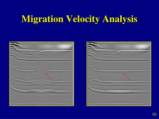
Migration velocity analysis by recursive wavefield extrapolation. Paul Sava & Biondo Biondi Stanford University SEP. Motivation. Wave-equation MVA (WEMVA). Band-limited Multi-pathing Resolution Born approximation small anomaly Rytov approximation phase unwrapping.

E N D
Migration velocity analysis by recursive wavefield extrapolation Paul Sava & Biondo Biondi Stanford University SEP paul@sep.stanford.edu
Motivation paul@sep.stanford.edu
Wave-equation MVA (WEMVA) Band-limited Multi-pathing Resolution Born approximation small anomaly Rytov approximation phase unwrapping paul@sep.stanford.edu
Wave-equation MVA (WEMVA) WE tomography data space WE MVA image space paul@sep.stanford.edu
Outline • WEMVA overview • Born image perturbation • Differential image perturbation • Example paul@sep.stanford.edu
A tomography problem paul@sep.stanford.edu
WEMVA: main idea paul@sep.stanford.edu
Born approximation paul@sep.stanford.edu
WEMVA: objective function Linear WEMVA operator slownessperturbation image perturbation (known) slowness perturbation (unknown) image perturbation paul@sep.stanford.edu
WEMVA: objective function paul@sep.stanford.edu
Fat ray: GOM example paul@sep.stanford.edu
Outline • WEMVA overview • Born image perturbation • Differential image perturbation • Example paul@sep.stanford.edu
“Data” estimate paul@sep.stanford.edu
Prestack Stolt residual migration r R0 R • Background image R0 • Velocity ratio r paul@sep.stanford.edu
Prestack Stolt residual migration r R0 R • Image perturbation paul@sep.stanford.edu
Born approximation paul@sep.stanford.edu
Residual migration: the problem Correct velocity Incorrect velocity Zero offset image Zero offset image Angle gathers Angle gathers paul@sep.stanford.edu
Born approximation paul@sep.stanford.edu
Outline • WEMVA overview • Born image perturbation • Differential image perturbation • Example paul@sep.stanford.edu
Differential image perturbation Image difference Image differential Computed Measured paul@sep.stanford.edu
Differential image perturbation R Rr R0 r r0 r paul@sep.stanford.edu
Phase perturbation Df +3p +2p +p 0 r -p -2p paul@sep.stanford.edu
Differential image perturbation paul@sep.stanford.edu
Born approximation paul@sep.stanford.edu
Example: background image Zero offset image Background image Angle gathers paul@sep.stanford.edu
Example: differential image Zero offset image Differential image Angle gathers paul@sep.stanford.edu
Example: slowness inversion Image perturbation Slowness perturbation paul@sep.stanford.edu
Example: updated image Updated image Updated slowness paul@sep.stanford.edu
Example: correct image Correct image Correct slowness paul@sep.stanford.edu
Outline • WEMVA overview • Born image perturbation • Differential image perturbation • Example paul@sep.stanford.edu
Field data example • North Sea • Salt environment • Subset • One non-linear iteration • Migration (background image) • Residual migration (image perturbation) • Slowness inversion (slowness perturbation) • Slowness update (updated slowness) • Re-migration (updated image) depth location paul@sep.stanford.edu
depth location depth paul@sep.stanford.edu
depth velocity ratio velocity ratio paul@sep.stanford.edu
depth location depth paul@sep.stanford.edu
depth location location paul@sep.stanford.edu
depth location location paul@sep.stanford.edu
depth location depth paul@sep.stanford.edu
depth location depth paul@sep.stanford.edu
Summary • MVA • Wavefield extrapolation methods • Born linearization • Differential image perturbations • Key points • Band-limited (sharp velocity contrasts) • Multi-pathing (complicated wavefields) • Resolution (frequency redundancy) paul@sep.stanford.edu
MVA information (a) g g x x z z paul@sep.stanford.edu
MVA information (b) g g x x z z paul@sep.stanford.edu
MVA information (c) w w g g paul@sep.stanford.edu
WEMVA cost reduction Full image Offset focusing Spatial focusing Frequency Normal incidence image Spatial focusing “fat” rays w w g g paul@sep.stanford.edu
Another example paul@sep.stanford.edu
Example: correct model Zero offset image Angle gathers paul@sep.stanford.edu
Example: background model Zero offset image Angle gathers paul@sep.stanford.edu
Example: correct perturbation Zero offset image Angle gathers paul@sep.stanford.edu
Example: differential perturbation Zero offset image Angle gathers paul@sep.stanford.edu
Example: perturbations comparison Correct Difference Differential paul@sep.stanford.edu