Download
1 / 32
510 likes | 1.09k Views
Velocity Analysis Jacobian. University of Bridgeport. Introduction to ROBOTICS. 1. Kinematic relations. X=FK( θ). θ = IK(X). Task Space. Joint Space. Location of the tool can be specified using a joint space or a cartesian space description. Velocity relations.

E N D
Velocity AnalysisJacobian University of Bridgeport Introduction to ROBOTICS 1
Kinematic relations X=FK(θ) θ =IK(X) Task Space Joint Space Location of the tool can be specified using a joint space or a cartesian space description
Velocity relations Relation between joint velocity and cartesian velocity. JACOBIAN matrix J(θ) Task Space Joint Space
Jacobian • Suppose a position and orientation vector of a manipulator is a function of 6 joint variables: (from forward kinematics) X = h(q)
Jacobian Matrix Forward kinematics
Jacobian Matrix Jacobian is a function of q, it is not a constant!
Linear velocity Angular velocity Jacobian Matrix The Jacbian Equation
(x , y) 2 l2 l1 1 Example • 2-DOF planar robot arm • Given l1, l2 ,Find: Jacobian
Singularities • The inverse of the jacobian matrix cannot be calculated when det [J(θ)] = 0 • Singular points are such values of θ that cause the determinant of the Jacobian to be zero
V (x , y) l2 Y 2 =0 l1 1 x • Find the singularity configuration of the 2-DOF planar robot arm determinant(J)=0 Not full rank Det(J)=0
Jacobian Matrix • Pseudoinverse • Let A be an mxn matrix, and let be the pseudoinverse of A. If A is of full rank, then can be computed as:
Jacobian Matrix Example: Find X s.t. Matlab Command: pinv(A) to calculate A+
Jacobian Matrix • Inverse Jacobian • Singularity • rank(J)<n : Jacobian Matrix is less than full rank • Jacobian is non-invertable • Boundary Singularities: occur when the tool tip is on the surface of the work envelop. • Interior Singularities: occur inside the work envelope when two or more of the axes of the robot form a straight line, i.e., collinear
Singularity • At Singularities: • the manipulator end effector cant move in certain directions. • Bounded End-Effector velocities may correspond to unbounded joint velocities. • Bounded joint torques may correspond to unbounded End-Effector forces and torques.
Jacobian Matrix • If • Then the cross product
Remember DH parmeter • The transformation matrix T
Jacobian Matrix (x , y) 2 l2 l1 1 • 2-DOF planar robot arm • Given l1, l2 ,Find: Jacobian • Here, n=2,
Jacobian Matrix (x , y) 2 l2 l1 1 • 2-DOF planar robot arm • Given l1, l2 ,Find: Jacobian • Here, n=2
Jacobian Matrix • The required Jacobian matrix J
Stanford Manipulator The DH parameters are:
Stanford Manipulator T4 = [ c1c2c4-s1s4, -c1s2, -c1c2s4-s1*c4, c1s2d3-sin1d2] [ s1c2c4+c1s4, -s1s2, -s1c2s4+c1c4, s1s2d3+c1*d2] [-s2c4, -c2, s2s4, c2*d3] [ 0, 0, 0, 1]
Stanford Manipulator T5 = [ (c1c2c4-s1s4)c5-c1s2s5, c1c2s4+s1c4, (c1c2c4-s1s4)s5+c1s2c5, c1s2d3-s1d2] [ (s1c2c4+c1s4)c5-s1s2s5, s1c2s4-c1c4, (s1c2c4+c1s4)s5+s1s2c5, s1s2d3+c1d2] [ -s2c4c5-c2s5, -s2s4, -s2c4s5+c2c5, c2d3] [ 0, 0, 0, 1]
Stanford Manipulator T5 = [ (c1c2c4-s1s4)c5-c1s2s5, c1c2s4+s1c4, (c1c2c4-s1s4)s5+c1s2c5, c1s2d3-s1d2] [ (s1c2c4+c1s4)c5-s1s2s5, s1c2s4-c1c4, (s1c2c4+c1s4)s5+s1s2c5, s1s2d3+c1d2] [ -s2c4c5-c2s5, -s2s4, -s2c4s5+c2c5, c2d3] [ 0, 0, 0, 1]
Stanford Manipulator T6 = [ c6c5c1c2c4-c6c5s1s4-c6c1s2s5+s6c1c2s4+s6s1c4, -c5c1c2c4+s6c5s1s4+s6c1s2s5+c6c1c2s4+c6s1c4, s5c1c2c4-s5s1s4+c1s2c5, d6s5c1c2c4-d6s5s1s4+d6c1s2c5+c1s2d3-s1d2] [ c6c5s1c2c4+c6c5c1s4-c6s1s2s5+s6s1c2s4-s6c1c4, -s6c5s1c2c4-s6c5c1s4+s6s1s2s5+c6s1c2s4-c6c1c4, s5s1c2c4+s5c1s4+s1s2c5, d6s5s1c2c4+d6s5c1s4+d6s1s2c5+s1s2d3+c1d2] [ -c6s2c4c5-c6c2s5-s2s4s6, s6s2c4c5+s6c2s5-s2s4c6, -s2c4s5+c2c5, -d6s2c4s5+d6c2c5+c2d3] [ 0, 0, 0, 1]
Stanford Manipulator Joints 1,2 are revolute Joint 3 is prismatic The required Jacobian matrix J
Inverse Velocity The relation between the joint and end-effector velocities: where j (m×n). If J is a square matrix (m=n), the joint velocities: If m<n, let pseudoinverse J+ where
Acceleration The relation between the joint and end-effector velocities: Differentiating this equation yields an expression for the acceleration: Given of the end-effector acceleration, the joint acceleration