Download
1 / 22
220 likes | 392 Views
Migration Velocity Analysis of Multi-source Data. Xin Wang January 7, 2010. 01. Outline. Motivation. Estimate an accurate background velocity model for multi-source migration. Theory. Tomographic migration velocity analysis method and least squares migration of multi-source data.

E N D
Migration Velocity Analysis of Multi-source Data Xin Wang January 7, 2010 01
Outline • Motivation • Estimate an accurate background velocity model for multi-source migration • Theory • Tomographic migration velocity analysis method and least squares migration of multi-source data. • Numerical Results • Synthetic tests of 2, 10 and 40 shot supergather on part of the 2D SEG/EAGE overthrust model. • Conclusions 02
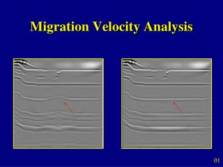
Motivation Inversion methods are sensitive to the background velocity model. True Velocity KM image CIG km/s 0 6 0 0 Seismic Data Z (km) Z (km) Z (km) 0 1.5 1.5 1.5 9 Time (s) 0 X (km) 6.4 0 X (km) 6.4 0 Offset (km) 2 Incorrect Velocity KM image m/s CIG 6.5 0 0 0 3 Z (km) Z (km) 1 Z (km) Trace # 160 1.5 1.5 1.5 9.5 0 X (km) 6.4 X (km) 6.4 0 0 Offset (km) 2 03
Motivation Multi-source technique reduces the economic cost of seismic acquisition. Single CSG 1 Supergather Single CSG 2 0 0 0 Time (s) Time (s) Time (s) 8 8 8 1 Trace # 129 129 1 Trace # 1 Trace # 129 Migration and stacking can suppress the cross-talk noise. (Hampson 2008, and Dai 2009). KM Image of 2 Shot Supergather LSM Image of 320 Shot Supergather 0 0 Z (km) Z (km) 1.3 1.3 0 0 X (km) 5.8 X (km) 5.8 Goal: can we apply the MVA method to multi-source data ? 04
Outline • Motivation • Estimate an accurate background velocity model for multi-source migration • Theory • Tomographic migration velocity analysis method and least squares migration of multi-source data. • Numerical Results • Synthetic tests of 2, 10 and 40 shot supergather on part of the 2D SEG/EAGE overthrust model. • Conclusions 05
Theory Layer stripping (Lafond, 1993) Shallow events are first flattened by updating shallow velocity layers by MVA, then deeper ones are flattened by updating deeper velocity. CIG CIG 0 0 Tomographic MVA Z0 Z (km) Z (km) Zh h 1.5 1.5 -1 Offset (km) 1 -1 Offset (km) 1 Hyperbolic approximation picking depth, zero-offset depth Depth residual reference depth With the eikonal solver, convert depth residual to time residual 06
Theory Traveltime tomography raypath operator, traveltime, background slowness. For a small slowness perturbation Parameterize the model as a grid of cells traveltime residual for the raypath , slowness purturbation in grid cell Back project along the raypaths to get Update the slowness with a steepest descent method 07
Theory Misfit function picked depth residual for offset in CIG of the iteration This value is used to help to determine when the iteration will stop. Multi-source data delay operator With a small number of multi-source, Kirchhoff migration is used With a large number of multi-source, least squares migration is used to suppress the crosstalk noise to provide a better image. 08
Theory Work Flow: All events are flattened? Go to the next curved event. Start from the top curved event. Y MVA finished ! Migration velocity model sk Migration velocity model s0 Y Predict travel time by eikonal solver KM for small N, form CIGs LSM for large N, form CIGs Flattened ? Pick the depth residual automatically Pick the reflector position from zero-offset and near-offset Find ray paths connecting the reflector to both S and R positions Convert depth residual to travel time residual Update velocity model by back projecting the traveltime residuals along the raypaths. 09
Outline • Motivation • Estimate an accurate background velocity model for multi-source migration • Theory • Tomographic migration velocity analysis method and least squares migration of multi-source data. • Numerical Results • Synthetic tests of 2, 10 and 40 shot supergather on part of the 2D SEG/EAGE overthrust model. • Conclusions 10
Numerical Results Part of 2D SEG/EAGE Overthrust model Size: 200 X 100 Interval: 25m Rick wavelet: central frequency 30 Hz, total source number: 200 km/s True Velocity Model Reflectivity Model 0.11 4.9 0 0 2D SEG/EAGE Overthrust Model Depth (km) Depth (km) 0 Depth (km) 2.5 -0.11 2.5 2.2 0 X (km) 10 Inaccurate Velocity Model Velocity Difference m/s km/s 0 4.9 0 0 Depth (km) Depth (km) 4.5 0 X (km) 10 -400 2.5 2.5 2.2 11 0 0 X (km) 10 X (km) 10
Numerical Results 2 Shot Supergather Initial Velocity model KM of 2 Shot Supergather CIG of KM with Initial Velocity km/s 0 0 4.9 0.6 Depth (km) Depth (km) Depth (km) 2.5 2.5 2.5 2.2 0 5 0 5 X (km) X (km) 0 3 Offset (km) Updated Velocity after Three Iterations of MVA CIG of KM with Updated Velocity KM of 2 Shot Supergather km/s 0 0 4.9 0.6 Depth (km) Depth (km) Depth (km) 2.5 2.5 2.5 2.2 0 3 Offset (km) 0 5 0 5 X (km) X (km) 12
Numerical Results 2 Shot Supergather Updated Velocity Difference after One Iterations of MVA Initial Velocity Difference m/s m/s 0 0 500 500 Depth (km) Depth (km) 0 0 2.5 2.5 0 5 0 5 X (km) X (km) Updated Velocity Difference after Two Iterations of MVA Updated Velocity Difference after Three Iterations of MVA m/s m/s 0 0 500 500 Depth (km) Depth (km) 0 2.5 2.5 0 0 5 X (km) 0 5 X (km) 13
Numerical Results 10 Shot Supergather Initial Velocity Model KM of 10 Shot Supergather CIG of KM with Initial Velocity km/s 0 0 4.9 0.6 Depth (km) Depth (km) Depth (km) 2.5 2.5 2.5 2.2 0 5 X (km) 0 5 0 3 X (km) Offset (km) Updated Velocity after Three Iterations of MVA CIG of KM with Updated Velocity KM of 10 Shot Supergather km/s 0 0 4.9 0.6 Depth (km) Depth (km) Depth (km) 2.5 2.5 2.5 2.2 0 3 Offset (km) 0 5 0 5 X (km) X (km) 14
Numerical Results 10 Shot Supergather Updated Velocity Difference after One Iterations of MVA Initial Velocity difference m/s m/s 0 0 500 500 Depth (km) Depth (km) 0 0 2.5 2.5 0 5 X (km) 0 5 X (km) Updated Velocity Difference after Two Iterations of MVA Updated Velocity Difference after Three Iterations of MVA m/s m/s 0 0 500 500 Depth (km) Depth (km) 0 0 2.5 2.5 0 5 X (km) 0 5 X (km) 15
Numerical Results 40 Shot Supergather CIG of LSM with Initial Velocity Initial Velocity Model LSM of 40 Shot Supergather km/s 0 0 4.9 0.6 Depth (km) Depth (km) Depth (km) 2.5 2.5 2.2 2.5 0 5 X (km) 0 5 0 3 X (km) Offset (km) Updated Velocity Model after Three Iterations of MVA CIG of LSM with Updated Velocity LSM of 40 Shot Supergather km/s 0 0 4.9 0.6 Depth (km) Depth (km) Depth (km) 2.5 2.5 2.5 2.2 0 3 Offset (km) 0 5 0 5 X (km) X (km) 16
Numerical Results 40 Shot Supergather Updated Velocity Difference after One Iterations of MVA Initial Velocity Difference m/s m/s 0 0 760 760 Depth (km) Depth (km) 0 0 2.5 2.5 0 5 0 5 X (km) X (km) Updated Velocity Difference after Two Iterations of MVA Updated Velocity Difference after Three Iterations of MVA m/s m/s 0 0 760 760 Depth (km) Depth (km) 0 0 2.5 2.5 X (km) 0 5 0 5 X (km) 17
Numerical Results 40 Shot Supergather LSM Data Residual with Updated Velocity by MVA 1.0 Normalized Data Residual 0.4 1 LSM Iteration Number 15 Depth Residual in CIG 1.0 Normalized Depth Residual 0 0 MVA Iteration Number 3 18
Outline • Motivation • Estimate an accurate background velocity model for multi-source migration • Theory • Tomographic migration velocity analysis method and least squares migration of multi-source data. • Numerical Results • Synthetic tests of 2, 10 and 40 shot supergather on part of the 2D SEG/EAGE overthrust model. • Conclusions 19
Conclusions • Tomographic MVA can be applied to multi-source seismic data. • MVA by KM is efficient with a small number of multi-source. • With a large number of multi-source, LSM is preferred. • After several iterations of updating, the depth residual reduces to • almost zero, although the updated velocity is still not • completely true. • When the multi-source number becomes to even larger , • the crosstalk in CIG prevents the MVA method. 20
Conclusions • Future Work: • Improve the LSM result with proper preconditioners (deblurring • filter) . • Apply some filters (F-K filter, slant-stacking and median filter) to • remove the incoherent noise in CIG for large multi-source number. • Use the reflection ray tracing method for dipping events. • Develop MVA for complicated synthetic model. 21
Acknowledgement We would like to thank the UTAM 2009 sponsors for their support. Thank You 22