Download
1 / 1
10 likes | 159 Views
Reconstructing ocean 3-d structure from surface measurements. Bruno Buongiorno Nardelli, Olga Cavalieri, Rosalia Santoleri, Marie-Helene Rio Gruppo di Oceanografia da Satellite Istituto di Scienze dell’Atmosfera e del Clima-Sezione di Roma, CNR Contact: bruno@gos.ifa.rm.cnr.it

E N D
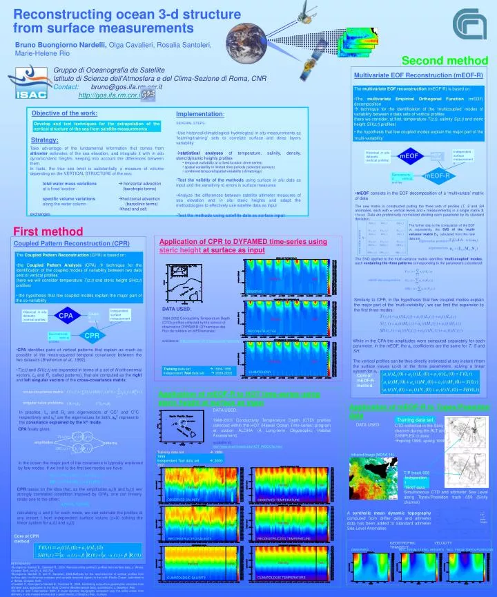
Reconstructing ocean 3-d structure from surface measurements Bruno Buongiorno Nardelli, Olga Cavalieri, Rosalia Santoleri, Marie-Helene Rio Gruppo di Oceanografia da Satellite Istituto di Scienze dell’Atmosfera e del Clima-Sezione di Roma, CNR Contact:bruno@gos.ifa.rm.cnr.it http://gos.ifa.rm.cnr.it/ Second method Multivariate EOF Reconstruction (mEOF-R) • The multivariate EOF reconstruction (mEOF-R) is based on: • The multivariate Empirical Orthogonal Function (mEOF) decomposition • technique for the identification of the ‘multicoupled’ modes of variability between n data sets of vertical profiles • (here we consider, at first, temperature T(z,t), salinity S(z,t) and steric height SH(z,t) profiles) • the hypothesis that few coupled modes explain the major part of the ‘multi-variability’ Objective of the work: Implementation: • SEVERAL STEPS: • Use historical/climatological hydrological in situ measurements as ‘learning/training’ sets to correlate surface and deep layers variability • statistical analyses of temperature, salinity, density, steric/dynamic heights profiles • temporal variability at a fixed location (time series) • spatial variability in limited time periods (selected surveys) • combined temporal/spatial variability (climatology) • Test the validity of the methods using surface in situ data as input and the sensitivity to errors in surface measures • Analyze the differences between satellite altimeter measures of sea elevation and in situ steric heights and adapt the methodologies to effectively use satellite data as input • Test the methods using satellite data as surface input Develop and test techniques for the extrapolation of the vertical structure of the sea from satellite measurements Strategy: Take advantage of the fundamental information that comes from altimeter estimates of the sea elevation, and integrate it with in situ dynamic/steric heights, keeping into account the differences between them. In facts, the true sea level is substantially a measure of volume depending on the VERTICAL STRUCTURE of the sea: total water mass variations horizontal advection at a fixed location(barotropic terms) specific volume variationshorizontal advection along the water column(baroclinic terms) heat and salt exchanges Independent surface measurements Historical in situ datasets (vertical profiles) mEOF mEOF modes mEOF-R Reconstructed vertical profiles • mEOF consists in the EOF decomposition of a ‘multivariate’ matrix of data • The new matrix is constructed putting the three sets of profiles (T, S and SH anomalies, each with m vertical levels and n measurements) in a single matrix X(3mn). Data are preliminarily normalized dividing each parameter by its standard deviation. The further step is the computation of the EOFor, equivalently, the SVD of the ‘multi-variance’ matrix Xcalculated from this new data set. First method XU=U U=(uk) Application of CPR to DYFAMED time-series using steric height at surface as input eigenvalue problem Coupled Pattern Reconstruction (CPR) new data matrix eigenvectors • The Coupled Pattern Reconstruction (CPR) is based on: • the Coupled Pattern Analysis (CPA) technique for the identification of the coupled modes of variability between two data sets of vertical profiles • (here we will consider temperature T(z,t) and steric height SH(z,t) profiles) • the hypothesis that few coupled modes explain the major part of the co-variability The SVD applied to the multi-variance matrix identifies ‘multi-coupled’ modes, each containing the three patterns corresponding to the parameters considered: training test mEOF decomposition OBSERVED Similarly to CPR, in the hypothesis that few coupled modes explain the major part of the ‘multi-variability’,we can limit the expansion to the first three modes: DATA USED: 1994-2002 Conductivity Temperature Depth (CTD) profiles collected by the service of observation DYFAMED (DYnamique des Flux de mAtière en MEDiterranée) Independent surface measurements Historical in situ datasets (vertical profiles) CPA Coupled modes training test RECONSTRUCTED CPR Reconstructed vertical profiles available at: http://www.obs-vlfr.fr/jgofs2/sodyf/hydro.htm While in the CPA the amplitudes were computed separately for each parameter, in the mEOF, the ak coefficients are the same for T, S and SH. The vertical profiles can be thus directly estimated at any instant t from the surface values (z=0) of the three parameters, solving a linear system for a1, a2 and a3: • CPA identifies pairs of vertical patterns that explain as much as possible of the mean-squared temporal covariance between the two datasets (Brethertonet al., 1992). • T(z,t) and SH(z,t) are expanded in terms of a set of N orthonormal vectors, Lk and Rk (called patterns), that are computed as the right and left singular vectors of the cross-covariance matrix: training test Training data set 1994-1999 Independent Test data set 2000-2002 CLIMATOLOGY Core of mEOF-R method Application of mEOF-R to HOT time-series using steric height at surface as input cross-covariance matrix singular value problems CRk=skLk CTLk=skRk Application of mEOF-R to Topex/Poseidon data In practice, Lk and Rk are eigenvectors of CCT and CTC respectively and sk2 are the eigenvalues for both. sk2represents the covariance explained by the kth mode. DATA USED: 1988-2001 Conductivity Temperature Depth (CTD) profiles collected within the HOT (Hawaii Ocean Time-series) program at station ALOHA (A Long-term Oligotrophic Habitat Assessment) Training data set DATA USED: • CTD collected in the Sicily channel during the ALT and SYMPLEX cruises • spring 1996, spring 1998 CPA finallygives: amplitudes available at: http://www.soest.hawaii.edu/HOT_WOCE/ftp.html patterns Infrared Image (NOAA-14) Training data set 1988-1999 Independent Test data set 2000-2001 In the ocean the major part of the covariance is typically explained by few modes. If we limit to the first two modes we have: T/P track 059 Independent TEST data training test training test CPR bases on the idea that, as the amplitudes ak(t) and bk(t) are strongly correlated (condition imposed by CPA), one can linearly relate one to the other: Simultaneous CTD and altimeter Sea Level along Topex/Poseidon track 059 (Sicily channel) OBSERVED SALINITY OBSERVED TEMPERATURE ak(t)=k·bk(t)+k calculating and for each mode, we can estimate the profiles at any instant t from independent surface values (z=0) solving the linear system for a1(t) and a2(t): A synthetic mean dynamic topography computed from drifter data and altimeter data has been added to Standard altimeter Sea Level Anomalies T/P ……∆ steric heights training test training test Core of CPR method RECONSTRUCTED TEMPERATURE RECONSTRUCTED SALINITY GEOSTROPHIC VELOCITY TRANSECT OBSERVED REC. FROM STERIC HEIGHTS REC. FROM TOPEX/POSEIDON training test training test • REFERENCES: • Buongiorno Nardelli B., Santoleri R., 2004. Reconstructing synthetic profiles from surface data, J. Atmos. Oceanic Tech., vol.21, 4, 693-703. • Buongiorno Nardelli B. and R. Santoleri, 2004:Methods for the reconstruction of vertical profiles from surface data: multivariate analyses and variable temporal signals in the north Pacific Ocean, submitted to J. Atmos. Oceanic Tech. • Cavalieri O., Buongiorno Nardelli B., Santoleri R., 2004. Estimating subsurface geostrophic velocities from altimeter data: application to the Sicily Channel (Mediterranean Sea), submitted to J. Geophys. Res. • Rio M.-H. and F.Hernandez, 2004: A mean dynamic topography computed over the world ocean from altimetry, in situ measurements and a geoid model, J.Geophys.Res., in press. CLIMATOLOGIC TEMPERATURE CLIMATOLOGIC SALINITY