Download
1 / 46
580 likes | 1.35k Views
Surface Mapping. Surface Mapping. Statistical surface Concept of a statistical surface Mapping the statistical surface with point, line and area symbols Portraying the land-surface form. Statistical surface. The statistical surface is one of the most important concepts in cartography.

E N D
Surface Mapping • Statistical surface • Concept of a statistical surface • Mapping the statistical surface with point, line and area symbols • Portraying the land-surface form Surface Mapping
Statistical surface • The statistical surface is one of the most important concepts in cartography. • The magnitudes of the attribute values, referenced to unit areas, lines or points, can be viewed as having a vertical dimension. • The magnitudes can therefore be visualised as a 3-dimensional surface. Surface Mapping
Concepts of statistical surface Left: An array of attribute values for unit areas. The numbers are rural population densities for minor civil divisions in a part of Kansas. Right: Elevated points whose relative height above the datum for each unit area is proportional to the attribute value in that unit area shown on the left. From Robinson, et al., 1995 Surface Mapping
Continuous and non-continuous surfaces Left: A perspective view of a smoothed statistical surface produced by assuming gradients among all the attribute values. Right: A perspective view of the statistical surface produced by erecting prisms over each unit area proportional in height to the attribute values. From Robinson, et al., 1995 Surface Mapping
2-D representations by isarithmic and choropleth maps Up: An isarithmic map of the statistical surface. Right: A choropleth representation of the same data set using 5 range-graded categories. From Robinson, et al., 1995 Surface Mapping
Mapping the statistical surface with point symbols • Dot map • Unit value • Size • Location A well-rendered dot map in which each dot represents 16.2 hectares of land in potato production. From Robinson, et al., 1995 Surface Mapping
Mapping the statistical surface with line symbols • Hachures: short line symbols whose width or spacing depends upon the slope at a point on the statistical surface. • Profiles: the lines of intersection between the series of parallel planes intersecting the datum at the right angle. • Oblique traces: intersects between 0 to 90°. • Isarithms: parallel to the datum. Surface Mapping
Hachures Line symbolisation of slopes or gradients by using hachures. In this diagram, hachures are equally spaced but vary in thickness depending on the value of the gradient being portrayed. Cited in Robinson, et al., 1995 Surface Mapping
Hachures (cont.) Benoit Bonne Hossard Line symbolisation of slopes or gradients by using hachures. In this diagram, hachures are of equal thickness but vary in spacing depending on the value of the gradient being portrayed. Cited in Robinson, et al., 1995 Surface Mapping
Profiles A series of profiles situated at right angles to one another gives a clear picture of the surface and its underlying strata. Cited in Robinson, et al., 1995 Surface Mapping
Construction of a profile The construction of a profile from an isarithmic map. Line AB is drawn on the map. Intersections of the isarithms with line AB are perpendicularly projected to the appropriate line of a set of parallel ruled lines below. The resulting points are connected by a smooth line resulting in a profile A’B’. From Robinson, et al., 1995 Surface Mapping
Oblique traces A reduced portion of a planimetrically correct terrain drawing of the Isle of Yell (Shetland Group). Cited in Robinson, et al., 1995 Surface Mapping
Perspective traces a b Perspective traces: (a) “fishnets” where traces are drawn in both the x and y directions, (b) traces drawn only parallel to the x direction, (c) traces drawn only parallel to the y direction. From Robinson, et al., 1995 c Surface Mapping
Perspective traces (cont.) Two sets of perspective traces: (a) suing one-point perspective, and (b) using two-point perspective. From Robinson, et al., 1995 Surface Mapping
Isarithmic mapping • An isarithm is also called isoline or isogram. • Emphasise on the geographical distribution outside surface enclosing the geographical volume. • Focus is on the attribute values at points of a truly continuous distribution. Surface Mapping
Isarithmic mapping (cont.) In the upper diagram, horizontal levels of given z values are seen passing partway through a hypothetical island. Traces of intersections of the planes with the island surface are indicated by dotted lines. In the lower drawing, the traces have been mapped orthogonally on the map datum and represent the island by means of isarithms. From Robinson, et al., 1995 Surface Mapping
Kinds of isarithmic mapping • Attribute values that can occur at points • Isometric lines • Attribute values that cannot occur at a point • Isopleths Surface Mapping
Mapping the statistical surface with area symbols • Choroplethic mapping • Simple choropleth mapping • Classless choropleth mapping • Elements of choroplethic mapping • Size and shapes of unit areas • Number of classes • Class limit determination • Dasymetric mapping Surface Mapping
Choroplethic mapping Examples of three ways we can map a set of z values that refer to enumeration districts or unit areas: (a) a simple choropleth map, (b) a dasymetric map, and (c) an isoplethic map. From Robinson, et al., 1995 Surface Mapping
> 40 25 - 40 10 - 25 < 10 Size and shape of unit areas A B The same distribution mapped with three different sets of unit areas, using the same class interval scheme: (a) uses large units of equal area, (b) uses small units of equal area, and (c) uses irregularly size unit areas. From Robinson, et al., 1995 C Surface Mapping
Number of classes A B Both (a) and (b) show five classes. Because of the simple distribution pattern on (a), we could increase the number of classes used. The lack of pattern in the distribution of (b) would make it even more confusing to the map reader if more classes were used. Cited in Robinson, et al., 1995 Surface Mapping
Class interval series (cont.) Left: An unclassed perspective view of a statistical distribution. Each unit area is shown as a prism whose height is proportional to the value of the mapped distribution, and whose base is a scaled representation of the unit area. Right: A five-classed, perspective view of the same statistical distribution. Cited in Robinson, et al., 1995 Surface Mapping
Choropleth map Surface Mapping
Portraying the land-surface form • Historical background • Visualisation methods • Terrain unit maps and hachures • Morphometric maps • Contouring • Hill shading • Perspective pictorial maps • Oblique regional views • Schematic maps Surface Mapping
Early maps Examples of portraying hills and mountains in stylised form on early maps. From Robinson, et al., 1995 Surface Mapping
Landform portrayal “From the 15th to 18th centuries, landform portrayal developed along with landscape painting of the period. Thus, perspective-like, oblique, or bird’s-eye views for limited areas became popular”. Cited in Robinson, et al., 1995 Surface Mapping
Landform portraying Chinese ancient maps also shows excellent art works in landscape portraying. Surface Mapping
Terrain unit maps A section of topographic map that portrays the land-surface form with vertically illuminated hachuring. Cited in Robinson, et al., 1995 Surface Mapping
Terrain unit maps and hachures A section of topographic map that portrays the land-surface form with obliquely illuminated hachuring. Cited in Robinson, et al., 1995 Surface Mapping
Morphometric maps On the left is a relatively realistic portrayal of the region. On the right is the same area, which employs a schematic treatment to emphasise the geomorphic characteristics Cited in Robinson, et al., 1995 Surface Mapping
Contouring Surface Mapping
A simple contour map Surface Mapping
Binary contour Surface Mapping
Altitude tinting Surface Mapping
Hill shading Courtesy www.hear.org/starr/maps/stock/index.html Surface Mapping
Hill-shaded topographic map “Recent printed topographic maps which combine hill shading with contours are the most effective ever produced by manual methods”. Cited in Robinson, et al., 1995 Surface Mapping
To see to believe? Left: hill-shaded topography with the illumination source located in the South – the real-world simulation for the North Hemisphere. On this image, the landform appears inversed. Right: the upside-down view of the same image. Surface Mapping
Hypsometric colouring (layer tinting) Surface Mapping Courtesy www.scilands.de
Layer tinting with contours Surface Mapping Courtesy geology.csustan.edu
Block diagrams “Even the simplest block diagram is easily accepted as a reduced replica of reality and is remarkably graphic”. From Robinson, et al., 1995 Surface Mapping
Oblique regional views A reduced preliminary “worksheet” of an oblique regional view of Europe as seen from the southwest, to illustrate a strategic viewpoint during the World War II. Cited in Robinson, et al., 1995 Surface Mapping
Perspective view with hill shade Shaded 3-dimensional landscape(courtesy http://hirise.lpl.arizona.edu/HiBlog/tag/dtm/). Surface Mapping
Perspective view with hill shade and shadow Surface Mapping
Perspective pictorial maps 3-dimensional surface draped with airphoto to show the 3-dimensional landscape – Ap Lei Chau, Hong Kong. Surface Mapping
Visual effects Visual effects can also be added for visualising the 3-dimensional surface more realistically (sky colours, clouds, etc.) – Ap Lei Chau, Hong Kong. Surface Mapping