Download
1 / 35
430 likes | 513 Views
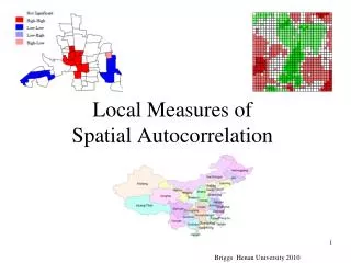
Global Measures of Spatial Autocorrelation. China. Last Time The concept of spatial autocorrelation. “Near things are more similar than distant things” The use of the weights matrix W ij to measure “nearness” The difficulty of measuring “nearness” This was a surprise! This Time

E N D
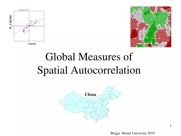
Global Measures ofSpatial Autocorrelation China Briggs Henan University 2010
Last Time • The concept of spatial autocorrelation. • “Near things are more similar than distant things” • The use of the weights matrix Wijto measure “nearness” • The difficulty of measuring “nearness” • This was a surprise! This Time • Measures of Spatial Autocorrelation • Join Count Statistic • Moran’s I • Geary’s C • Getis-Ord G statistic Briggs Henan University 2010
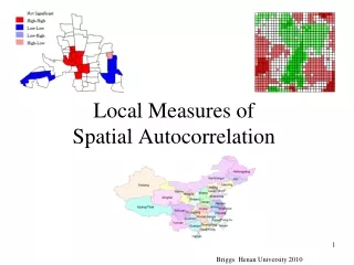
Global Measures and Local Measures China An equivalent local measure can be calculated for most global measures • Global Measures • A single value which applies to the entire data set • The same pattern or process occurs over the entire geographic area • An average for the entire area • Local Measures • A value calculated for each observation unit • Different patterns or processes may occur in different parts of the region • A unique number for each location Briggs Henan University 2010
Join (or Joins or Joint) Count Statistic • Polygons only • binary (1,0) data only • Polygon has or does not have a characteristic • For example, a candidate won or lost an election • Based on examining polygons which share a border • Do they have the same characteristic or not? • Border same on each side • Border not the same on each side • Requires a contiguity matrix for polygons Briggs Henan University 2010
Join (or Joint or Joins) Count Statistic • Uses binary (1,0) data • Shown here as B/W (black/white) • Measures the number of borders (“joins”) of each type (1,1), (0,0), (1,0 or 0,1) relative to total number of borders • For 6 x 6 matrix, border totals are: • 60 for Rook Case • 110 for Queen Case Small number of BW joins (6 only for rook) Large proportion of BB and WW joins Different numbers of BW, BB and WW joins Large number of BW joins Small number of BB and WW joins Briggs Henan University 2010
Join Count: Test Statistic Expected = random pattern generated by tossing a coin in each cell. Test Statistic given by: Z= Observed - Expected SD of Expected Standard Deviation of Expected (standard error) given by: Expected given by: Where: k is the total number of joins (neighbors) pB is the expected proportion Black, if random pW is the expected proportion White m is calculated from k according to: Note: the formulae given here are for free (normality) sampling. Those for non-free (randomization) sampling are substantially more complex. See Wong and Lee 1st ed. p. 151 compared to p. 155. Se next slide for explanation. Briggs Henan University 2010
A Note on Sampling Assumptions:applies to most tests for spatial autocorrelation • Test results depend on the assumption made regarding the type of sampling: • Free (or normality) sampling • Analogous to sampling with replacement • After a polygon is selected for a sample, it is returned to the population set • The same polygon can occur more than one time in a sample • Non-free (or randomization) sampling • Analogous to sampling without replacement • After a polygon is selected for a sample, it is not returned to the population set • The same polygon can occur only one time in a sample • The formulae used to calculate the test statistic (particularly the standard error) are different for each • Generally, the formulae are substantially more complex for free sampling—unfortunately, it is also the more common situation! • Assuming free sampling requires knowledge about larger trends from outside the region or access to additional information within the region in order to estimate parameters. Briggs Henan University 2010
Gore/Bush Presidential Election 2000 Is there evidence of clustering by State? Use Join Count to answer this question! Many BB joins total number of joins = 109 = sum of neighbors/2 in the sparse contiguity matrix = number of 1s/2 in the full contiguity matrix for US States (see slides from SA Concepts lecture) Briggs Henan University 2010
Queens Case Sparse Contiguity Matrix for US States • Ncount is the number of neighbors for each state • Equals number of 1s in a row of full contiguity matrix • Sum of Ncount is 218 • Number of common borders (joins) = • ncount / 2 = 109 • N1, N2… FIPS codes for neighbors Briggs Henan University 2010
Join Count Statistic for Gore/Bush 2000 by State • The expected number of joins is calculated based on the proportion of votes each received in the election (for Bush = 109*.499*.499=27.125) • K = 109= total number of joins • There are far more Bush/Bush joins (actual = 60) than would be expected (27) • Since test score (3.79) is greater than the critical value (2.54 at 1%) result is statistically significant at the 99% confidence level (p <= 0.01) • Strong evidence of spatial autocorrelation—clustering • There are far fewer Bush/Gore joins (actual = 28) than would be expected (54) • Since test score (-5.07) is greater than the critical value (2.54 at 1%) result is statistically significant at 99% confidence level (p <= 0.01) • Again, strong evidence of spatial autocorrelation—clustering • Actual calculations available in spatstat.xls spreadsheet (JC-%vote tab) Briggs Henan University 2010
UNIFORM/ DISPERSED CLUSTERED Moran’s I • The most common measure of Spatial Autocorrelation • Use for points or polygons • Join Count statistic only for polygons • Use for a continuous variable (any value) • Join Count statistic only for binary variable (1,0) • Varies on a scale between –1 through 0* to + 1 -1 0 +1 *technically it is: –1/(n-1) high negative spatial autocorrelation no spatial autocorrelation* high positive spatial autocorrelation Can also use it as an index for dispersion/random/cluster patterns. Dispersed Pattern Random Pattern Clustered Pattern Briggs Henan University 2010
Moran’s I and Correlation Coefficient rDifferences and Similarities Crime in nearby area Income Correlation Coefficient r • Relationship between two variables r = 0.71 or Crime Rate Education Grocery Store Density Nearby r = -0.71 r = -0.71 Quantity Price • Moran’s I • Involves one variable only • Correlation between variable, X, and the “spatial lag” of X formed by averaging all the values of X for the neighboring polygons Grocery Store Density r = 0.71 Briggs Henan University 2010
Formula for Moran’s I • Where: N is the number of observations (points or polygons) is the mean of the variableXi is the variable value at a particular locationXj is the variable value at another locationWij is a weight indexing location of i relative to j Briggs Henan University 2010
CorrelationCoefficient Note the similarity of the numerator (top) to the measures of spatial association discussed earlier if we view Yi as being the Xi for the neighboring polygon (see next slide) = Spatial auto-correlation Briggs Henan University 2010
CorrelationCoefficient Spatial weights Yi is the Xi for the neighboring polygon = Moran’s I Briggs Henan University 2010
Adjustment for Short or Zero Distances • If an inverse distance measure is used, and distances are very short, then wij becomes very large and distorts I. • An adjustment for short distances can be used, usually scaling the distance to one mile. • The units in the adjustment formula are the number of data measurement units in a mile • In the example, the data is assumed to be in feet. • With this adjustment, the weights will never exceed 1 • If a contiguity matrix is used (1or 0 only), this adjustment is unnecessary Briggs Henan University 2010
Where: I is the calculated value for Moran’s I from the sample E(I) is the expected value if random S is the standard error Statistical Significance Tests for Moran’s I • Based on the normal frequency distribution with E(I) = -1/(n-1) • Again, there are two different formula for calculating the standard error • The free sampling or normality method • The nonfree sampling or randomization method • These formulae are complicated! • They are in Lee and Wong 1st Ed. p. 82 and 160-1 • In either case, the statistical test is carried out in the same way Briggs Henan University 2010
1% 2.5% 2.5% 1.96 2.54 -1.96 0 Test Statistic for Normal Frequency Distribution *technically –1/(n-1) –1/(n-1) Reject null Reject null at 5% Null Hypothesis: no spatial autocorrelation *Moran’s I = 0 Alternative Hypothesis: spatial autocorrelation exists *Moran’s I > 0 Reject Null Hypothesis if Z test statistic > 1.96 (or < -1.96) ---less than a 5% chance that, in the population, there is no spatial autocorrelation ---95% confident that spatial auto correlation exits Reject null at 1%
Null Hypothesis: no spatial autocorrelation *Moran’s I = 0 Alternative Hypothesis: spatial autocorrelation exists *Moran’s I > 0 Reject Null Hypothesis if Z test statistic > 1.96 (or < -1.96) ---less than a 5% chance that, in the population, there is no spatial autocorrelation ---95% confident that spatial auto correlation exits Briggs Henan University 2010
Moran Scatter Plots Moran’s I can be interpreted as the correlation between variable, X, and the “spatial lag” of X formed by averaging all the values of X for the neighboring polygons We can then draw a scatter diagram between these two variables (in standardized form): X and lag-X (or W_X) Lag Xi is average of these Xi Least squares “best fit” line to the points. The slope of this regression line is Moran’s I (will discuss Regression later) Briggs Henan University 2010
Moran Scatterplot: example Moran’s I = 0.49 Lag-X High surrounded by high Low surrounded by low X Population density in Puerto Rico • Scatterplot of X vs. Lag-X • The slope of the regression line is Moran’s I GISC 7361 Spatial Statistics
Moran’s I for rate-based data • Moran’s I is often calculated for rates, such as crime rates (e.g. number of crimes per 1,000 population) or infant mortality rates (e.g. number of deaths per 1,000 births) • An adjustment should be made, especially if the denominator in the rate (population or number of births) varies greatly (as it usually does) • Adjustment is know as the EB adjustment: • see Assuncao-Reis Empirical Bayes StandardizationStatistics in Medicine, 1999 • GeoDA software includes an option for this adjustment Briggs Henan University 2010
Geary’s C (Contiguity) Ratio • Calculation is similar to Moran’s I, • For Moran, the cross-product is based on the deviations from the mean for the two location values • For Geary, the cross-product uses the actual values themselves at each location • Interpretation is very different, essentially the opposite! Geary’s C varies on a scale from 0 to 2 • 0 indicates perfect positive autocorrelation/clustered • 1 indicates no autocorrelation/random • 2 indicates perfect negative autocorrelation/dispersed • Can convert to a -/+1 scale by: calculating C* = 1 - C • Moran’s I usually used! Briggs Henan University 2010
Statistical Significance Tests for Geary’s C Where: C is the calculated value for Geary’s C from the sample E(C) is the expected value if no autocorrelation S is the standard error • Similar to Moran • Again, based on the normal frequency distribution with however, E(C) = 1 • Again, there are two different formulations for the standard error calculation • The randomization or nonfree sampling method • The normality or free sampling method • The actual formulae for calculation are in Lee and Wong, 1st Ed. p. 81 and p. 162 Briggs Henan University 2010
Hot Spots and Cold Spots e.g. high crime area e.g. low crime area • Moran’s I and Geary’s C cannot distinguish them • They only indicate clustering • Cannot tell if these are hot spots, cold spots, or both • What is a hot spot? • A place where high values cluster together • What is a cold spot? • A place where low values cluster together Briggs Henan University 2010
Getis-Ord General/Global G-Statistic • The G statistic distinguishes between hot spots and cold spots. It identifies spatial concentrations. • G is relatively large if high values cluster together • G is relatively low if low values cluster together • The General G statistic is interpreted relative to its expected value • The value for which there is no spatial association • G > (larger than) expected value potential “hot spots” • G < (smaller than) expected value potential “cold spots” • A Z test statistic is used to test if the difference is statistically significant • Calculation of G based on a neighborhood distance within which cluster is expected to occur Getis, A. and Ord, J.K. (1992) The analysis of spatial association by use of distance statistics Geographical Analysis, 24(3) 189-206 Briggs Henan University 2010
where Calculating General G Where: d is neighborhood distance Wij weights matrix has only 1 or 0 1 if j is within d distance of i 0 if its beyond that distance Thus any point beyond distance d has a value of zero and therefore is excluded d • Begins by identifying a distance band, d, within which clustering occurs • Actual Value for G is given by: • the terms in the numerator (top) are calculated “within a distance ring (d),” and are then divided by totals for the entire region to create a proportion • if nearby x values are both large (indicating “hot” spot), the numerator (top) will be large • If they are both small (indicating “cold” spot), the numerator (top) will be small • Expected value for G (if no concentration) is given by: Number of points within distance band d Total number of points in study region Briggs Henan University 2010
Comments on General G • General G will not show negative spatial autocorrelation • Should only be calculated for ratio scale data • data with a “natural” zero such as crime rates, birth rates • Although it was defined using a contiguity (0,1) weights matrix, any type of spatial weights matrix can be used • ArcGIS gives multiple options • There are two global versions: G and G* • G does not include the value of Xi itself, only “neighborhood” values • G* includes Xi as well as “neighborhood” values Briggs Henan University 2010
with Testing General G • The test statistic for G is normally distributed and is given by: • The next slide shows the results for running General G on Anselin’s Columbus crime data • This data is not good, but is very common since Anselin uses it in his original LISA article and in the examples in the GeoDA documentation • The geographic coordinates are completely arbitrary Calculation of the standard error is complex. See Lee and Wong 1st pp 164-167 or Getis and Ord 1992 for formulae. Briggs Henan University 2010
General/Global G in ArcGIS Shapefile containing polygon or point data Variable to analyze Different options available for specifying cluster neighborhood --simple distance band selected, as described in lecture Options for measuring distance --straight line (Euclidean) --city block Size of neighborhood distance band Briggs Henan University 2010
General/Global G in ArcGIS: results Observed G = .777 Expected G = .637 Observed > Expected >> “Hot spots” Z score: 5.067 > 1.96 >> significant But where are the hot spots? For this we use Local Statistics Briggs Henan University 2010
What have we learned today? • Difference between global and local measures of spatial autocorrelation • How to calculate and interpret some global measures • Join Count Statistic • Used for binary (0,1) data only • Moran’s I • The most common global measure of spatial autocorrelation • Geary’s C • interpretation almost opposite of Moran’s I, but not used very often • Getis-Ord G statistic • Identifies hot spots or cold spots Next Time: local measures of spatial autocorrelation Briggs Henan University 2010
Challenge for You Calculate Moran’s I and/or General G for some appropriate variables in the China provinces data set Use ArcGIS or GeoDA software Briggs Henan University 2010
References • O’Sullivan and Unwin Geographic Information Analysis New York: John Wiley, 1st ed. 2003, 2nd ed. 2010 • Jay Lee and David Wong Statistical Analysis with ArcView GIS New York: Wiley, 1st ed. 2001 (all page references are to this book), 2nd ed. 2005 • Unfortunately, these books are based on old software (Avenue scripts used with ArcView 3.x) and no longer work in the current version of ArcGIS 9 or 10. • Ned Levine and Associates CrimeStat III Washington: National Institutes of Justice, 2010 • Available as pdf • download from: http://www.icpsr.umich.edu/NACJD/crimestat.html Briggs Henan University 2010