Download
1 / 19
210 likes | 543 Views
Autocorrelation. Lecture 19. Today’s plan. Durbin’s h-statistic Autoregressive Distributed Lag model & Finite Lags Koyck Transformation Testing in the presence of higher order serially correlated forms. Seasonality

E N D
Autocorrelation Lecture 19
Today’s plan • Durbin’s h-statistic • Autoregressive Distributed Lag model & Finite Lags • Koyck Transformation • Testing in the presence of higher order serially correlated forms. • Seasonality • (Note: should also look at Chapter 13 of the book: Stock and Watson as well as indicated parts of Chapter 12 from the reading list).
Returning to the Durbin-Watson • Last time we talked about how to test for autocorrelation using the Durbin-Watson test • We found autocorrelation in the model in L_18.xls: Yt = a + bXt + et • DW test gave figure of 0.331. DL critical value= 1.475 • Reject H0: r = 0 • Indication of positive first order autocorrelation. • Note, no lagged regressors in the model. • If we reject null - need an estimate for r for generalized least squares estimation.
Generalized least squares • Need an estimate of : we can transform the variables such that: where: • Known as Cochrane-Orcutt transformation. • Notice that describes the relationship between neighboring errors in the model. • Estimating equation (3) allows us to estimate in the presence of first-order autocorrelation
Problems 1) The model presented by may still have some autocorrelation • the D-W test doesn’t tell us anything about this • we have to retest the model 2) We may lose information when we lag our variables • to get around this information loss, we can use the Prais-Winsten formula to transform the model:
Problems (2) 3) We might want to include a lagged endogenous variable in the model • including the lagged endogenous variable Yt-1 biases the Durbin-Watson test towards 2 • this means it’s biased towards the null of no autocorrelation • in this instance, we’ll use Durbin’s h-statistic (1970): v = square of the standard error on the coefficient (g) of the lagged endogenous variable
Durbin’s h-statistic • Durbin’s h-statistic is normally distributed and is approximated by the z-statistic (standard normal) • null hypothesis: H0: = 0 • the null can be rejected at (say) the 5% level of significance • L19.xls has example. • Problems with the h-statistic • the product nv must be less than one (where n = # of observations) • if nv 1, the h-statistic is undefined
A note on consistency • Model with lagged endogenous variable and first-order serially correlated error may be mis-specified. Yt = b0 + b1Yt-1 + ut and ut = rut-1 + et • If so, presence of first-order serial correlation may induce omitted variable bias. • Need to include additional lagged endogenous variable term: Yt = a0 + a1Yt-1 + a2Yt-2 + et
Why lags? • This mainly relates to macroeconomic models • economic events such as consumer expenditure, production, or investment • for instance: consumer expenditure this year may be related to consumer expenditure last year • In a general distributed lag model: Yt = a + g1Yt-1 +…+ g2Yt-p + b0Xt + b1Xt-1 +…+bkXt-q + et • where p,q = lag length: note problems for degrees of freedom • can eliminate coefficients by using a t-test (or joint test using F).
Why lags? (2) • Number of lags included is ad-hoc. • Test on Causality (does the X cause Y) by using the Granger causality test. F-test on b1 to bq equaling zero. • Known as an ADL(p,q) (autoregressive distributed lag) model of order p on dependent, q on independent. • Lags lead to severe problems for ordinary least squares • loss of information (degrees of freedom) • independent variables (X) are highly correlated [multi-collinearity problem]
Why lags are useful • Psychological reasons: behavior is habit-forming • so things like labor market behavior and patterns of money holding can be captured using lags • Technological reasons: a firm’s production pattern • Institutional: unions • Multipliers: short run and long run multipliers (how to read finite distributed lags in a model).
Ad-hoc nature of lags • What can we do? • Two approaches • Transform the model (e.g. Koyck) • Use of information criterion • Both approaches have costs and benefits
Koyck transformation • Model: Yt = a + b0Xt + b1Xt-1 +…+bkXt-k + et • Note: no lagged variables on the dependent variable. • The Koyck transformation suggests that the further back in time we go, the less important is that factor • for instance, information from 10 years ago vs. information from last year • The transformation suggests: Where 0 < < 1 j = 1,…k
Koyck transformation (2) • So, • Can use the expression for bj to rewrite the model Yt = a + b0 (Xt + Xt-1 + 2Xt-2 + ….+ kXt-k) + et(4) • this imposes the assumption that earlier information is relatively less important • Lagging the equation and multiplying it by , we get: Yt-1 = a + b0 (Xt-1 + 2Xt-2 + ….+ kXt-k) + et-1 (5) • Subtracting (5) from (4), we get Yt = a(1- ) + b0Xt + Yt-1 + vt where vt = et - et-1
Koyck transformation (3) • Why is this transformation useful? • Allows us to take the ad-hoc lag series (on independent variable) and condense it into a lagged endogenous variable • now we only lose one observation due to the lagged endogenous variable • the given by transform provides estimate of r • Problem: by construction, we have first-order autocorrelation • use Durbin h-statistic • but estimating equation might be mis-specified!
Information Criterion • Determining the order of autoregression (inclusion of lagged values of Y) or the lag length for the variables in the model (the order p and q for the ADL). • Same formula for both (known as Bayes or Schwartz Information Criterion): • BIC(p) = ln(SSR(p)/T) + (p+1)(lnT/T) • As lags on dependent variable increase (up to pmax), SSR (sum of squared residuals) decreases. The term starting (p+1) increases. • Trade-off one against the other: need BIC at a minimum. • Same principle for q lags on independent variable.
Problems with the approaches • How do we know model of economic behavior represented by Koyck actually occurs? Estimating form of model can have other interpretations (e.g. adaptive expectations) • Koyck gives 1st-order autocorrelation by the construction of the model (use the Durbin h-statistic). If autocorrelation detected, transform model and estimate by GLS • Yt-1 and et-1 (ut-1) are sure to be correlated [ E(X,e) 0] • this leads to biased estimates • we’ll deal with this using instrumental variables and simultaneous equations
Problems with the approaches • ADL model gives no idea of how many lags should be included despite the BIC. What do we do if the number of observations does not allow optimal lag lengths to be included? • Problem of lags inducing collinearity between regressors. Even if we removed problems of autocorrelation, multicollinearity may bias estimates of the variances!
Other topics • Testing and correcting in the presence of higher orders of serial correlation. • Seasonality and the use of dummy variables in time series models. • Trends and their use in time series models