Spatial Autocorrelation Basics NR 245 Austin Troy University of Vermont

1. Spatial Autocorrelation BasicsNR 245Austin TroyUniversity of Vermont

2. SA basics • Lack of independence for nearby obs • Negative vs. positive vs. random • Induced vs inherent spatial autocorrelation • Induced when thing being measured is a function of the actual autocorrelated variable • First order (gradient) vs. second order (patchiness) • SA can be at two scales: within patch and between patch • Directional patterns: anisotropy • Measured based on point pairs

3. Spatial lags Source: ESRI, ArcGIS help

4. Statistical ramifications • Spatial version of redundancy • If the observations are spatially clustered the estimates obtained from the correlation coefficient or OLS estimator will be biased and confidence intervals too narrow. • biased because the areas with higher concentration of events will have a greater impact on the model estimate and they will overestimate precision because, since events tend to be concentrated, there are actually fewer number of independent observations than degrees of freedom indicate. Like measuring the same thing many times • estimate of the standard errors will be too low. This might lead you to believe that some coefficients are significant, when in fact they are not. False positives or Type 1 errors • End up with systematic bias in models towards variables that are correlated in space • Similar to pseudo-replication in ecology

5. Example • Example from Prof Allan Frei: “Imagine if you had data from 10 counties spread all over the northeast. The data includes variables such as median income, # of highways, and access to the internet. You regress access to the internet (dependent variable) against the other two (independent) variables. You realize that n=10 is not enough to get significant results, so you need more data. So, you go get data from 10 additional counties, but you choose the counties that are immediately adjacent to the original 10. If incomes and infrastructure hardly change from one county to the next, you are not really getting any additional information. This would be spatial autocorrelation. So how does this affect the regression results? You would be doing the calculations as if you had n=20 cases, but in reality you only had 10 independent cases. So, you would be overestimating the number of degrees of freedom, getting unrealistic t and p values, and underestimating the standard errors of the coefficients.” Source: http://www.geography.hunter.cuny.edu/~afrei/gtech702_fall03_webpages/notes_spatial_autocorrelation.htm

6. Tests • Null hypothesis: observed spatial pattern of values is equally likely as any other spatial pattern • Test if values observed at a location do not depend on values observed at neighboring locations

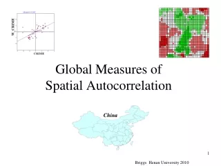
7. Moran’s I • Ratio of two expressions: similarity of pairs, including only those within distance threshold adjusted for number of items, over variance of data • Applied to zones or points with continuous variables associated with them. • Compares the value of the variable at any one location with the value at all other locations Where N is the number of casesXi is the variable value at a particular locationXj is the variable value at another location is the mean of the variableWij is a weight applied to the comparison between location i and location j OR # of connections In matrix See http://www.spatialanalysisonline.com/output/html/MoranIandGearyC.html#_ref177275168 for more detail

8. Moran’s I • Wij is a contiguity matrix • If zone j is adjacent to zone i, the interaction receives a weight of 1: see lags from second slide • Another option is to make Wij a distance-based weight which is the inverse distance between locations I and j (1/dij) • Or can use both (this is an option in ArcGIS) • Compares the sum of the cross-products of values at different locations, two at a time weighted by the inverse of the distance between the locations • Varies between –1.0 and + 1.0 • When autocorrelation is high, the coefficient is high • A high I value indicates positive autocorrelation • Significance tested with Z statistic

9. Geary’s C • One prob with Moran’s I is that it’s based on averages so easily biased by skewed distribution with outliers. • Geary’s C deals with this because: • Interaction is not the cross-product of the deviations from the mean like Moran, but the deviations in intensities of each observation location with one another • However it can also be biased in presence of skewness but for another reason; squared differences between one value and an outlier value will have disproportionate effect on index

10. Geary’s C • Value typically range between 0 and 2 • If value of any one zone are spatially unrelated to any other zone, the expected value of C will be 1 • Values less than 1 (between 1 and 2) indicate negative spatial autocorrelation • Inversely related to Moran’s I • Does not provide identical inference because it emphasizes the differences in values between pairs of observations, rather than the covariation between the pairs. • Moran’s I gives a more global indicator, whereas the Geary coefficient is more sensitive to differences in small neighborhoods.

11. Scale effects • Can measure I or C at different spatial lags to see scale dependency with spatial correlogram Source:http://iussp2005.princeton.edu/download.aspx?submissionId=51529

12. Source: Fortin and Dale, Spatial Analysis

13. LISA • Local version of Moran: maps individual covariance components of global Moran • Require some adjustment: standardize row total in weight matrix (number of neighbors) to sum to 1—allows for weighted averaging of neighbors’ influence • Also use n-1 instead of n as multiplier • Usually standardized with z-scores • +/- 1.96 is usually a critical threshold value for Z And expected value where

14. Gwynns Fall Crime Data

15. Local Moran

16. Local Getis with 2000 m weights

17. Local Getis with adjacency weights

18. Local Getis-Ord Statistic • Used in Arc GIS • Indicates both clustering and whether clustered values are high or low • For a chosen critical distance d, G(d) is •  where xi is the value of ith point, w(d) is the weight for point i and j for distance d.