Download

1 / 44
770 likes | 1.78k Views
Spatial Autocorrelation and Spatial Regression. Elisabeth Root Department of Geography. A few good books…. Bivand , R., E.J. Pebesma and V. Gomez-Rubio. Applied Spatial Data Analysis with R . New York: Springer.

E N D
Spatial Autocorrelation and Spatial Regression Elisabeth Root Department of Geography
A few good books… • Bivand, R., E.J. Pebesma and V. Gomez-Rubio. Applied Spatial Data Analysis with R. New York: Springer. • Ward, M.D. and K.S. Gleditsch (2008). Spatial Regression Models. Thousand Oaks, CA: Sage.
First, a note on spatial data • Point data • Accuracy of location is very important • Area/lattice data • Data reported for some regular or irregular areal unit • 2 key components of spatial data: • Attribute data • Spatial data
Tobler’s First Law of Geography • “All places are related but nearby places are more related than distant places” • Spatial autocorrelation is the formal property that measures the degree to which near and distant things are related • Statistical test of match between locational similarity and attribute similarity • Positive, negative or zero relationship
Spatial regression Steps in determining the extent of spatial autocorrelation in your data and running a spatial regression: • Choose a neighborhood criterion • Which areas are linked? • Assign weights to the areas that are linked • Create a spatial weights matrix • Run statistical test to examine spatial autocorrelation • Run a OLS regression • Determine what type of spatial regression to run • Run a spatial regression • Apply weights matrix
Spatial weights matrices • Neighborhoods can be defined in a number of ways • Contiguity (common boundary) • What is a “shared” boundary? • Distance (distance band, K-nearest neighbors) • How many “neighbors” to include, what distance do we use? • General weights (social distance, distance decay)
Step 1: Choose a neighborhood criterion Importing shapefiles into R and constructing neighborhood sets
R libraries we’ll use SET YOUR CRAN MIRROR > install.packages(“ctv”) > library(“ctv”) > install.views(“Spatial”) > library(maptools) > library(rgdal) > library(spdep) You only need to do this once on your computer
Importing a shapefile > library(maptools) > getinfo.shape("C:/Users/ERoot/Desktop/R/sids2.shp") Shapefile type: Polygon, (5), # of Shapes: 100 > sids<-readShapePoly ("C:/Users/ERoot/Desktop/R/sids2.shp") > class(sids) [1] "SpatialPolygonsDataFrame" attr(,"package")
Importing a shapefile (2) > library(rgdal) > sids<-readOGRdsn="C:/Users/ERoot/Desktop/R",layer="sids2") OGR data source with driver: ESRI Shapefile Source: "C:/Users/Elisabeth Root/Desktop/Quant/R/shapefiles", layer: "sids2" with 100 features and 18 fields Feature type: wkbPolygon with 2 dimensions > class(sids) [1] "SpatialPolygonsDataFrame" attr(,"package") [1] "sp"
Projecting a shapefile • If the shapefile has no .prj file associated with it, you need to assign a coordinate system > proj4string(sids)<-CRS("+proj=longlatellps=WGS84") • We can then transform the map into any projection > sids_NAD<-spTransform(sids, CRS("+init=epsg:3358")) > sids_SP<-spTransform(sids, CRS("+init=ESRI:102719")) • For a list of applicable CRS codes: • http://www.spatialreference.org/ref/ • Stick with the epsg and esri codes
Contiguity based neighbors • Areas sharing any boundary point (QUEEN) are taken as neighbors, using the poly2nb function, which accepts a SpatialPolygonsDataFrame > library(spdep) > sids_nbq<-poly2nb(sids) • If contiguity is defined as areas sharing more than one boundary point (ROOK), the queen= argument is set to FALSE > sids_nbr<-poly2nb(sids, queen=FALSE) > coords<-coordinates(sids) > plot(sids) > plot(sids_nbq, coords, add=T)
Queen Rook
Distance based neighborsk nearest neighbors • Can also choose the k nearest points as neighbors > coords<-coordinates(sids_SP) > IDs<-row.names(as(sids_SP, "data.frame")) > sids_kn1<-knn2nb(knearneigh(coords, k=1), row.names=IDs) > sids_kn2<-knn2nb(knearneigh(coords, k=2), row.names=IDs) > sids_kn4<-knn2nb(knearneigh(coords, k=4), row.names=IDs) > plot(sids_SP) > plot(sids_kn2, coords, add=T) k=2 k=1 k=3
k=1 k=2 k=4
Distance based neighborsSpecified distance • Can also assign neighbors based on a specified distance > dist<-unlist(nbdists(sids_kn1, coords)) > summary(dist) Min. 1st Qu. Median Mean 3rd Qu. Max. 40100 89770 97640 96290 107200 134600 > max_k1<-max(dist) > sids_kd1<-dnearneigh(coords, d1=0, d2=0.75*max_k1, row.names=IDs) > sids_kd2<-dnearneigh(coords, d1=0, d2=1*max_k1, row.names=IDs) > sids_kd3<-dnearneigh(coords, d1=0, d2=1.5*max_k1, row.names=IDs) OR by raw distance > sids_ran1<-dnearneigh(coords, d1=0, d2=134600, row.names=IDs)
dist=0.75*max_k1 (k=1) dist=1*max_k1=134600 dist=1.5*max_k1 dist=1*max_k1 dist=1.5*max_k1
Step 2: Assign weights to the areas that are linked Creating spatial weights matrices using neighborhood lists
Spatial weights matrices • Once our list of neighbors has been created, we assign spatial weights to each relationship • Can be binary or variable • Even when the values are binary 0/1, the issue of what to do with no-neighbor observations arises • Binary weighting will, for a target feature, assign a value of 1 to neighboring features and 0 to all other features • Used with fixed distance, k nearest neighbors, and contiguity
Row-standardized weights matrix > sids_nbq_w<- nb2listw(sids_nbq) > sids_nbq_w Characteristics of weights list: Neighbour list object: Number of regions: 100 Number of nonzero links: 490 Percentage nonzero weights: 4.9 Average number of links: 4.9 Weights style: W Weights constants summary: n nn S0 S1 S2 W 100 10000 100 44.65023 410.4746 • Row standardization is used to create proportional weights in cases where features have an unequal number of neighbors • Divide each neighbor weight for a feature by the sum of all neighbor weights • Obsi has 3 neighbors, each has a weight of 1/3 • Obs j has 2 neighbors, each has a weight of 1/2 • Use is you want comparable spatial parameters across different data sets with different connectivity structures
Binary weights > sids_nbq_wb<-nb2listw(sids_nbq, style="B") > sids_nbq_wb Characteristics of weights list: Neighbour list object: Number of regions: 100 Number of nonzero links: 490 Percentage nonzero weights: 4.9 Average number of links: 4.9 Weights style: B Weights constants summary: n nn S0 S1 S2 B 100 10000 490 980 10696 • Row-standardised weights increase the influence of links from observations with few neighbours • Binary weights vary the influence of observations • Those with many neighbours are up-weighted compared to those with few
Binary vs. row-standardized • A binary weights matrix looks like: • A row-standardized matrix it looks like:
Regions with no neighbors • If you ever get the following error: Error in nb2listw(filename): Empty neighbor sets found • You have some regions that have NO neighbors • This is most likely an artifact of your GIS data (digitizing errors, slivers, etc), which you should fix in a GIS • Also could have “true” islands (e.g., Hawaii, San Juans in WA) • May want to use k nearest neighbors • Or add zero.policy=T to the nb2listw call > sids_nbq_w<-nb2listw(sids_nbq, zero.policy=T)
Step 3: Examine spatial autocorrelation Using spatial weights matrices, run statistical tests of spatial autocorrelation
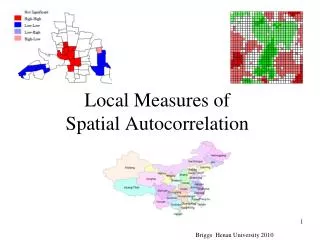
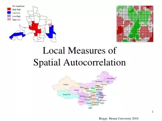
Spatial autocorrelation • Test for the presence of spatial autocorrelation • Global • Moran’s I • Geary’s C • Local (LISA – Local Indicators of Spatial Autocorrelation) • Local Moran’s I and GetisGi* • We’ll just focus on the “industry standard” – Moran’s I
Moran’s I in R > moran.test(sids_NAD$SIDR79, listw=sids_nbq_w, alternative=“two.sided”) Moran's I test under randomisation data: sids_NAD$SIDR79 weights: sids_nbq_w Moran I statistic standard deviate = 2.3625, p-value = 0.009075 alternative hypothesis: greater sample estimates: Moran I statistic Expectation Variance 0.142750392 -0.010101010 0.004185853 “two.sided” → HA: I ≠ I0 “greater” →HA: I >I0
Moran’s I in R > moran.test(sids_NAD$SIDR79, listw=sids_nbq_wb) Moran's I test under randomisation data: sids_NAD$SIDR79 weights: sids_nbq_wb Moran I statistic standard deviate = 1.9633, p-value = 0.02480 alternative hypothesis: greater sample estimates: Moran I statistic Expectation Variance 0.110520684 -0.010101010 0.003774597
Moving on to spatial regression Modeling data in R
Spatial autocorrelation in residualsSpatial error model • Incorporates spatial effects through error term • Where: • If there is no spatial correlation between the errors, then = 0
Spatial autocorrelation in DV Spatial lag model • Incorporates spatial effects by including a spatially lagged dependent variable as an additional predictor • Where: • If there is no spatial dependence, and y does no depend on neighboring y values, = 0
Spatial Regression in R • Read in boston.shp • Define neighbors (k nearest w/point data) • Create weights matrix • Moran’s test of DV, Moran scatterplot • Run OLS regression • Check residuals for spatial dependence • Determine which SR model to use w/LM tests • Run spatial regression model
Define neighbors and create weights matrix > boston<-readOGR(dsn="F:/R/shapefiles",layer="boston") > class(boston) > boston$LOGMEDV<-log(boston$CMEDV) > coords<-coordinates(boston) > IDs<-row.names(as(boston, "data.frame")) > bost_kd1<-dnearneigh(coords, d1=0, d2=3.973, row.names=IDs) > plot(boston) > plot(bost_kd1, coords, add=T) > bost_kd1_w<- nb2listw(bost_kd1)
Moran’s I on the DV > moran.test(boston$LOGMEDV, listw=bost_kd1_w) Moran's I test under randomisation data: boston$LOGMEDV weights: bost_kd1_w Moran I statistic standard deviate = 24.5658, p-value < 2.2e-16 alternative hypothesis: greater sample estimates: Moran I statistic Expectation Variance 0.3273430100 -0.0019801980 0.0001797138
Moran Plot for the DV > moran.plot(boston$LOGMEDV, bost_kd1_w, labels=as.character(boston$ID))
OLS Regression bostlm<-lm(LOGMEDV~RM + LSTAT + CRIM + ZN + CHAS + DIS, data=boston) Residuals: Min 1Q Median 3Q Max -0.71552 -0.11248 -0.02159 0.10678 0.93024 Coefficients: Estimate Std. Error t value Pr(>|t|) (Intercept) 2.8718878 0.1316376 21.817 < 2e-16 *** RM 0.1153095 0.0172813 6.672 6.70e-11 *** LSTAT -0.0345160 0.0019665 -17.552 < 2e-16 *** CRIM -0.0115726 0.0012476 -9.276 < 2e-16 *** ZN 0.0019330 0.0005512 3.507 0.000494 *** CHAS 0.1342672 0.0370521 3.624 0.000320 *** DIS -0.0302262 0.0066230 -4.564 6.33e-06 *** --- Residual standard error: 0.2081 on 499 degrees of freedom Multiple R-squared: 0.7433, Adjusted R-squared: 0.7402 F-statistic: 240.8 on 6 and 499 DF, p-value: < 2.2e-16
Checking residuals for spatial autocorrelation > boston$lmresid<-residuals(bostlm) > lm.morantest(bostlm, bost_kd1_w) Global Moran's I for regression residuals Moran I statistic standard deviate = 5.8542, p-value = 2.396e-09 alternative hypothesis: greater sample estimates: Observed Moran's I Expectation Variance 0.0700808323 -0.0054856590 0.0001666168
Determining the type of dependence > lm.LMtests(bostlm, bost_kd1_w, test="all") Lagrange multiplier diagnostics for spatial dependence LMerr = 26.1243, df = 1, p-value = 3.201e-07 LMlag = 46.7233, df = 1, p-value = 8.175e-12 RLMerr = 5.0497, df = 1, p-value = 0.02463 RLMlag = 25.6486, df = 1, p-value = 4.096e-07 SARMA = 51.773, df = 2, p-value = 5.723e-12 • Robust tests used to find a proper alternative • Only use robust forms when BOTH LMErr and LMLag are significant
One more diagnostic… > install.packages(“lmtest”) > library(lmtest) > bptest(bostlm) studentizedBreusch-Pagan test data: bostlm BP = 70.9173, df = 6, p-value = 2.651e-13 • Indicates errors are heteroskedastic • Not surprising since we have spatial dependence
Running a spatial lag model > bostlag<-lagsarlm(LOGMEDV~RM + LSTAT + CRIM + ZN + CHAS + DIS, data=boston, bost_kd1_w) Type: lag Coefficients: (asymptotic standard errors) Estimate Std. Error z value Pr(>|z|) (Intercept) 1.94228260 0.19267675 10.0805 < 2.2e-16 RM 0.10158292 0.01655116 6.1375 8.382e-10 LSTAT -0.03227679 0.00192717 -16.7483 < 2.2e-16 CRIM -0.01033127 0.00120283 -8.5891 < 2.2e-16 ZN 0.00166558 0.00052968 3.1445 0.001664 CHAS 0.07238573 0.03608725 2.0059 0.044872 DIS -0.04285133 0.00655158 -6.5406 6.127e-11 Rho: 0.34416, LR test value:37.426, p-value:9.4936e-10 Asymptotic standard error: 0.051967 z-value: 6.6226, p-value: 3.5291e-11 Wald statistic: 43.859, p-value: 3.5291e-11 Log likelihood: 98.51632 for lag model ML residual variance (sigma squared): 0.03944, (sigma: 0.1986) AIC: -179.03, (AIC for lm: -143.61)
A few more diagnostics LM test for residual autocorrelation test value: 1.9852, p-value: 0.15884 > bptest.sarlm(bostlag) studentizedBreusch-Pagan test data: BP = 60.0237, df = 6, p-value = 4.451e-11 • LM test suggests there is no more spatial autocorrelation in the data • BP test indicates remaining heteroskedasticity in the residuals • Most likely due to misspecification
Running a spatial error model > bosterr<-errorsarlm(LOGMEDV~RM + LSTAT + CRIM + ZN + CHAS + DIS, data=boston, listw=bost_kd1_w) Type: error Coefficients: (asymptotic standard errors) Estimate Std. Error z value Pr(>|z|) (Intercept) 2.96330332 0.13381870 22.1442 < 2.2e-16 RM 0.09816980 0.01700824 5.7719 7.838e-09 LSTAT -0.03413153 0.00194289 -17.5674 < 2.2e-16 CRIM -0.01055839 0.00125282 -8.4277 < 2.2e-16 ZN 0.00200686 0.00062018 3.2359 0.001212 CHAS 0.06527760 0.03766168 1.7333 0.083049 DIS -0.02780598 0.01064794 -2.6114 0.009017 Lambda: 0.59085, LR test value: 24.766, p-value: 6.4731e-07 Asymptotic standard error: 0.086787 z-value: 6.8081, p-value: 9.8916e-12 Wald statistic: 46.35, p-value: 9.8918e-12 Log likelihood: 92.18617 for error model ML residual variance (sigma squared): 0.03989, (sigma: 0.19972) AIC: -166.37, (AIC for lm: -143.61)