Download
1 / 44
610 likes | 1.38k Views
Inverting the Jacobian and Manipulability. Howie Choset (with notes copied from Rob Platt). The Inverse Problem. Quick review of linear algebra. Forward Kinematics is in general many to one (if more joint angles than DOF in WS), non linear

E N D
Inverting the Jacobianand Manipulability Howie Choset (with notes copied from Rob Platt)
The Inverse Problem Quick review of linear algebra Forward Kinematics is in general many to one (if more joint angles than DOF in WS), non linear Inverse Kinematics is in general one to many (have a choice), non linear Forward differential kinematics, linear, many to one, etc. based on # of DOF and WS Inverse is “easier” because linear, but this many to one issue comes up
The Inverse Problem Quick review of linear algebra
Cartesian control Let’s control the position (not orientation) of the three link arm end effector: We can use the same strategy that we used before:
Cartesian control joint ctlr joint position sensor However, this only works if the Jacobian is square and full rank… • All rows/columns are linearly independent, or • Columns span Cartesian space, or • Determinant is not zero
Cartesian control What if you want to control the two-dimensional position of a three-link manipulator? Two equations of three variables each… • This is an under-constrained system of equations. • multiple solutions • there are multiple joint angle velocities that realize the same EFF velocity.
Generalized inverse • If the Jacobian is not a square matrix (or is not full rank), then the inverse doesn’t exist… • what next? We have: We are looking for a matrix such that:
Generalized inverse • Two cases: • Underconstrained manipulator (redundant) • Overconstrained • Generalized inverse: • for the underconstrained manipulator: given , find any vector s.t. • for the overconstrained manipulator: given , find any vector s.t. Is minimized
Jacobian Pseudoinverse: Redundant manipulator Psuedoinverse definition: (underconstrained) Given a desired twist, , find a vector of joint velocities, , that satisfies while minimizing Minimize joint velocities Minimize subject to : Use lagrange multiplier method: This condition must be met when is at a minimum subject to
Jacobian Pseudoinverse: Redundant manipulator Minimize Subject to
Jacobian Pseudoinverse: Redundant manipulator I won’t say why, but if is full rank, then is invertible • So, the pseudoinverse calculates the vector of joint velocities that satisfies while minimizing the squared magnitude of joint velocity ( ). • Therefore, the pseudoinverse calculates the least-squares solution.
Calculating the pseudoinverse The pseudoinverse can be calculated using two different equations depending upon the number of rows and columns: Underconstrained case (if there are more columns than rows (m<n)) Overconstrained case (if there are more rows than columns (n<m)) If there are an equal number of rows and columns (n=m) These equations can only be used if the Jacobian is full rank; otherwise, use singular value decomposition (SVD):
Calculating the pseudoinverse using SVD Singular value decomposition decomposes a matrix as follows: is a diagonal matrix of singular values:
Properties of the pseudoinverse Moore-Penrose conditions: Generalized inverse: satisfies condition 1 Reflexive generalized inverse: satisfies conditions 1 and 2 Pseudoinverse: satisfies all four conditions Other useful properties of the pseudoinverse:
Controlling Cartesian Position joint ctlr joint position sensor • Procedure for controlling position: • Calculate position error: • Multiply by a scaling factor: • Multiply by the velocity Jacobian pseudoinverse:
Controlling Cartesian Orientation • How does this strategy work for orientation control? • Suppose you want to reach an orientation of • Your current orientation is • You’ve calculated a difference: • How do you turn this difference into a desired angular velocity to use in ? joint ctlr joint position sensor
Controlling Cartesian Orientation • You can’t do this: • Convert the difference to ZYZ Euler angles: • Multiply the Euler angles by a scaling factor and pretend that they are an angular velocity: Remember that in general: joint ctlr joint position sensor
The Analytical Jacobian If you really want to multiply the angular Jacobian by the derivative of an Euler angle, you have to convert to the “analytical” Jacobian: For ZYZ Euler angles Gimbal lock: by using an analytical Jacobian instead of the angular velocity Jacobian, you introduce the gimbal lock problems we talked about earlier into the Jacobian – this essentially adds “singularities” (we’ll talk more about that in a bit…)
Controlling Cartesian Orientation The easiest way to handle this Cartesian orientation problem is to represent the error in axis-angle format Axis angle delta rotation • Procedure for controlling rotation: • Represent the rotation error in axis angle format: • Multiply by a scaling factor: • Multiply by the angular velocity Jacobian pseudoinverse:
Controlling Cartesian Orientation • Why does axis angle work? • Remember Rodrigues’ formula from before: axis angle Compare this to the definition of angular velocity: The solution to this FO diff eqn is: Therefore, the angular velocity gets integrated into an axis angle representation
Jacobian Transpose Control • The story of Cartesian control so far:
Jacobian Transpose Control Start with a squared position error function (assume the poses are represented as row vectors) Here’s another approach: Position error: Gradient descent: take steps proportional to in the direction of the negative gradient.
Jacobian Transpose Control The same approach can be used to control orientation: orientation error: axis angle orientation of reference pose in the current end effector reference frame:
Jacobian Transpose Control So, evidently, this is the gradient of that • Jacobian transpose control descends a squared error function. • Gradient descent always follows the steepest gradient
Jacobian Transpose v Pseudoinverse • What gives? • Which is more direct? Jacobian pseudoinverse or transpose? or • They do different things: • Transpose: move toward a reference pose as quickly as possible • One dimensional goal (squared distance meteric) • Pseudoinverse: move along a least squares reference twist trajectory • Six dimensional goal (or whatever the dimension of the relevant twist is)
Jacobian Transpose v Pseudoinverse • The pseudoinverse moves the end effector in a straight line path toward the goal pose using the least squared joint velocities. • The goal is specified in terms of the reference twist • Manipulator follows a straight line path in Cartesian space • The transpose moves the end effector toward the goal position • In general, not a straight line path in Cartesian space • Instead, the transpose follows the gradient in joint space
Using the Jacobian for Statics Up until now, we’ve used the Jacobian in the twist equation, Interestingly, you can also use the Jacobian in a statics equation: Joint torques Cartesian wrench: force moment (torque)
When J is not invertible: Case 1 minimizes
Singularities for most configurations
Manipulability • A measure of the Jacobian • Configuration dependent • Maybe it is a measure of how far away from a singularity • Norms • Scalar • Vector • Matrix
Manipulability Ellipsoid Can we characterize how close we are to a singularity? Yes – imagine the possible instantaneous motions are described by an ellipsoid in Cartesian space. Can’t move much this way Can move a lot this way
Manipulability Ellipsoid The manipulability ellipsoid is an ellipse in Cartesian space corresponding to the twists that unit joint velocities can generate: A unit sphere in joint velocity space Project the sphere into Cartesian space The space of feasible Cartesian velocities
Manipulability Ellipsoid • You can calculate the directions and magnitudes of the principle axes of the ellipsoid by taking the eigenvalues and eigenvectors of • The lengths of the axes are the square roots of the eigenvalues • Yoshikawa’s manipulability measure: • You try to maximize this measure • Maximized in isotropic configurations • This measures the volume of the ellipsoid
Manipulability Ellipsoid • Another characterization of the manipulability ellipsoid: the ratio of the largest eigenvalue to the smallest eigenvalue: • Let be the largest eigenvalue and let be the smallest. • Then the condition number of the ellipsoid is: • The closer to one the condition number, the more isotropic the ellispoid is.
Manipulability Ellipsoid Isotropic manipulability ellipsoid NOT isotropic manipulability ellipsoid
Force Manipulability Ellipsoid You can also calculate a manipulability ellipsoid for force: A unit sphere in the space of joint torques The space of feasible Cartesian wrenches
Manipulability Ellipsoid • Principle axes of the force manipulability ellipsoid: the eigenvalues and eigenvectors of: • has the same eigenvectors as : • But, the eigenvalues of the force and velocity ellipsoids are reciprocals: • Therefore, the shortest principle axes of the velocity ellipsoid are the longest principle axes of the force ellipsoid and vice versa…
Velocity and force manipulability are orthogonal! Force ellipsoid Velocity ellipsoid • This is known as force/velocity duality • You can apply the largest forces in the same directions that your max velocity is smallest • Your max velocity is greatest in the directions where you can only apply the smallest forces
Manipulability Ellipsoid: Example Solve for the principle axes of the manipulability ellipsoid for the planar two link manipulator with unit length links at Principle axes:
Eigenvalues and Vectors • Eigenvectors are the directions that a linear mapping just scales a vector • Ax = sx where A is a matrix, s is a scalar • Det (Ax) = Det (sx) • Eigenvectors • Ellipsoid analogy
Singular Values • Eigenvalues are for squares (remember the determinant) • This square matrix has eigenvalues and vectors