Download
1 / 65
670 likes | 808 Views
ME 4135 Differential Motion and the Robot Jacobian. Fall 2012 R. R. Lindeke, Ph.D. Lets develop the differential Operator – bringing calculus to Robots. The Differential Operator is a way to account for “Tiny Motions” ( T)

E N D
ME 4135Differential Motion and the Robot Jacobian Fall 2012 R. R. Lindeke, Ph.D.
Lets develop the differential Operator – bringing calculus to Robots • The Differential Operator is a way to account for “Tiny Motions” (T) • It can be used to study movement of the End Frame over a short time interval (t) • It is a way to track and explain motion for different points of view
Considering motion: • We can define a General Rotation of a vector K: • By a general matrix defined as:
These Rotation are given as: • But lets remember, for our purposes that this angle is very small (a ‘tiny rotation’) • If the angle is small we can have some simplifications: • Cos small 1 • Sin small small
Substituting the Small angle Approximation: Similarly for Y and Z:
Simplifying the Rotation Matricies (product) Here, we have neglected products of the terms!
What about Small (general) Translation? • We define it as a matrix: • General Tiny Motion is then (both considering both Rotation and Translation):
So let’s use this idea: • Here we define a motion which is due to a robot’s joint(s) moving during a small time interval: • T+T = {Rot(K,d)*Trans(dx,dy,dz)}T • Note, T is the original pose • Substituting for the matrices:
Further Simplifying: We will call this matrix the del operator:
Thus, the Change in POSE (T) • dT(that is T) = T • = {[Trans(dx,dy,dz)*Rot(K,d)] – I} • Here we see that this operator is analagous to the derivative operator d( )/du when taken wrt HTM’s
Lets look into an application: • Given: • Subject it to 2 simultaneous movements: • Along X0 (dx) a translation of .0002 units (/unit time) • About Z0a Rotation of 0.001rad (/unit time)
Graphically: Here: Rinit = (32 + 52) .5 = 5.831 units init = Atan2(3,5) = 1.0304 rad R
Where is the Frame ‘n’ after one time step? • Considering Position: • Effect of “Translation”: • X=3.0002 and Y = 5.000 • New Rf = (3.00022 + 5.02).5 = 5.83105 u • Effect of Rotation • fin = 1.0304 + 0.001 = 1.0314 rad Xf= Cos(fin) * Rf = 2.99505 & Yf= Sin(fin) * Rf = 5.00309
Where is the Frame n after one time step? • Considering Orientation:
Lets Approximate it with the ‘ operator’ • Tnew = Tinit + dT = Tinit + Tinit • Where:
Comparing: • “Exact”: • Approximate: Realistically these are all but equal and using the ‘del’ approximation is soooo much easier!
We can (might!) use the ‘del’ approach to move a robot in space: • Take a starting POSE (Torig) & a starting motion set (deltas in rotation and translation as function of unit times) • Form operator for motion • Compute dT( Torig) • Form Tnew= Torig + dT • Repeat as time moves forward over the time steps …
Taking Motion WRT other Spaces (non inertial basis) • Original Model: • dT = T (1) • Motion Taken WRT another (non-inertia) space: • dT = TT (2) • Here T implies motion wrt its own frame but could be any other non-inertia space • But the change itself (dT) is independent of point of view so, equating (1) and (2) we can isolate T • T = (T)-1 T
Solving for the specific Terms in T • Origin Change Vector wrtTspace: • Angular effects wrtTspace: d, n, o& a vectors are extracts from the T Matrix dp is the translation vector in is the rotational effect in
Finding T -- from earlier example The Orientation Effects: Translation Effects:
Approximating New T Pose with the ‘ T operator’ • Tnew = Tinit + dT = Tinit + Tinit*T • Where:
Comparing: • “Exact” (from earlier): • New Approximation: Realistically these are all but equal – actually closer with this technique
An Application of this issue: TRpart TCamPart TWCR If the Part is moving along a conveyor and we “measure” its motion with a Camera (in camera frame) but we want to pick up the part with the robot, we must ‘track’ it so we need to known the part motion in robot’s space (not camera space!).
This is a Motion “Mapping” Issue: • Pa R WC Ca PaPa R C Pa • Pa R WC Ca Pa • Knowns: • C • Robot in WC • Camera in WC • And of course Part in Camera (But we don’t need it now!)
Lets Isolate the “Middle” • R WC CaR C • R WC Ca • To solve for R we “mathematically move” from R to R directly (R) and “The long way around”:
Rewriting into Standard Form: • It can be shown for any 2 Matrices (A & B): • A-1*B = (B-1*A)-1 (1) • If, on the previous page we consider: • TWCRas “A” and TWCCamas “B”, • And define (TWCCam)-1*(TWCR) as “T” • Now, Using the theorem above (from matrix math), then • We find that R = “T”-1(Cam )”T” • R is now shown in the standard form of earlier • the terms: d, n, s& a vectors in the “T” matrix and the dp and vectors from the Cam are then all that is required to define part motion with respect to the robot space
R is given by simplifying! • (TWCCam)-1*(TWCR) = “T” HERE: d, n, s& a vectors are extracts from the “T” Matrix above dp is the ‘translation’ vector in Cam is the ‘rotational effects’ in Cam Thus we would have a means for tracking a moving part directly into robot space!
Now, Lets Examine the Jacobian • Fundamentally: • We use these Jacobians to further our knowledge of Geometric Calculus
In This Model, Ddot& Dq,dot are: We state, then, that the Jacobian is a mapping tool that relates Cartesian Velocities (of the end frame) to the movement of the individual Robot Joints
Lets build one from ‘1st Principles’ – Here is a Spherical Arm: Lets start with only linear motion ---- its straight forward! R
Writing the Position Models: • Z = R*Sin() • X = R*Cos()*Cos() • Y = R*Cos()*Sin() To find velocity differentiate these which leads to:
Writing it as a Matrix: This is the linear motion Jacobian; It is built as the Matrix of partial joint contributions (coefficients of the velocity equations) to Velocity of the End Frame
Here we could develop an Inverse Jacobian: It was formed by taking the partial derivatives of the IKS eqns.
The process we did just now is limited to finding Linear Velocity • We need linear and angular velocity for full functional robots! • We can approach the problem by separations as before … • Here we had separated Velocity (Linear from Rotational) but not joints (arms) from joints (wrist) • Generally speaking, in the Jacobian we will obtain one Column for each Joint and 6 rows for full velocity effect • We say the Jacobian is a 6 by n matrix
Seperation Leads to: • A Cartesian Velocity Term V0n: • An Angular Velocity Term 0n: Each of these “Ji’s” are 3 Row by n Columned Matrices!
Building the Sub-Jacobians (in general): • We define 3 motion stipulations: • Velocities can only be added if they are defined in the same space • Motion of the end effecter (n frame) is taken wrt the base space (0 frame) • Linear Velocity effects are (truly) physically separated from angular velocity effects • To address the problem we will only move one joint at a time (uses the fundamental DH separation principle!)
Lets start with the Angular Velocity (!) • Considering any joint i, its Axis of motion is: Zi-1 (Z in Frame i-1) • The (modeling) effect of the joint is to drive the very next frame (frame i) • If Joint i is revolute: • here ki-1is the unit vector of Zi-1 • This could be applied to each of the joints (revolute) in the machine (it rotates the next frame – and of course, all subsequent frames rotate similarly!) • But if the Joint is Prismatic, it has no angular effect on its “controlled” frame (and, thus, subsequent frames all the way to the end frame)
Developing the J • We need to add up each of the joint effects • BUT, We need to “normalize” them to base space to added them up • DH methods allow us to do this! • Since Zi-1 is in a Frame of the model, we really need only extract the 3rd column of the product of A1* A2* …*Ai-1 to have a definition of Zi-1 in base space to add the effect of Joint i in this ‘common space’ (note, the ‘qdot’ term is the rotational velocity of the revolute joint)
So J then is just this: Note Zi-1 for Jointi – per DH algorithm! As stated previously, Zi-1 is the (1st 3 rows) of the 3rd col. of A0*…Ai-1 And we will have a term in the sum for each joint
For the Spherical Device: Notice: 3 cols. since we have 3 joints! All the rest of the Zi’s depend on the Frame Skeleton drawn!
Building the Linear Jacobian • It too will depend on the movement of Zi-1 • It too will require that we normalize each joints contribution to the base space • We will also find that revolute and prismatic joints will make functionally different contributions to the solution (as if we would think otherwise!) • Prismatics are “Easy,” Revolutes, not so much!
Building the Linear Jacobian – Prismatic Joints When the prismatic jointi moves, all subsequent links move (linearly) at the same rate and in the same direction
Building the Linear Jacobian – Prismatic Joints • Therefore, for each prismatic joint of a machine, the contribution to the Jacobian (after normalizing) is: • Zi-1 which is the 3rd column of the matrix given by: • A1* … * Ai-1 • This is as expected based on the model on the previous slide
Building the Linear Jacobian – Revolute Joints • This is a dicer problem – remembering the idea of prismatic joints on angular velocity … • But no that won’t work here • just because its a rotation, and it (primarily) changes orientation of the end, it does also have a linear contribution effect to the motion of the end as we saw in in our earlier “Del” discussion – that is revolute joints have a “levering effect” which moves the origin of the n-frame (and the levering is clearly a cartesian motion). • We must compute and account for this effect and then normalize it too.