Download
1 / 48
860 likes | 1.73k Views
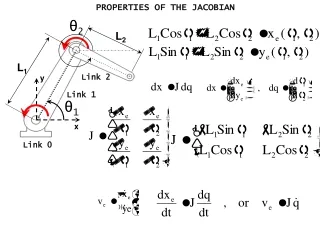
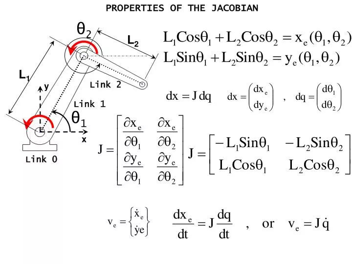
PROPERTIES OF THE JACOBIAN. θ 2. L 2. L 1. Link 2. y. Link 1. θ 1. x. Link 0. The Jacobian plays an important role in the analysis, design and control of robotic systems. The Jacobian can be expressed by its two coulmns. Then the velocity relation is given as follows.

E N D
PROPERTIES OF THE JACOBIAN θ2 L2 L1 Link 2 y Link 1 θ1 x Link 0
The Jacobian plays an important role in the analysis, design and control of robotic systems. The Jacobian can be expressed by its two coulmns Then the velocity relation is given as follows The first term on the right-hand side accounts for the end-effecter velocity induced by the first joint only, while the second term represents the velocity resulting from the second joint motion only. The resultant end-effecter velocity is given by the vectorial sum of the two. Each vector of the Jacobian matrix represents the end-effecter velocity generated by the corresponding joint moving at a unit velocity when all other joints are immobilized.
J1 θ2 L2 J2 L1 Link 2 y E Link 1 θ1 x Link 0 Figure illustrates the column vectors J1 and J2 of the 2 dof robot arm in the two dimensional space. Vector J2, given by the second column of the Jacobian matrix, points in the direction perpendicular to link 2. Note, however, that vector J1 is not perpendicular to link 1 but is perpendicular to line OE, the line from joint 1 to the endpoint E.
J1 represents the endpoint velocity induced by joint 1 when joint 2 is immobilized. In other words, links 1 and 2 are rigidly connected, becoming a single rigid body of link length OE, and J1 is the tip velocity of the link OE. In general, each column vector of the Jacobian represents the end-effecter velocity and angular velocity generated by the individual joint velocity while all other joints are immobilized. Let be the end-effecter velocity and angular velocity, or the end-effecter velocity for short, and Ji be the i-th column of the Jacobian. The end-effecter velocity is given by a linear combination of the Jacobian column vectors weighted by the individual joint velocities. where n is the number of active joints. The geometric interpretation of the column vectors is that J1 is the end-effecter velocity and angular velocity when all the joints other than joint i are immobilized and only the i-th joint is moving at a unit velocity.
Remember that the end-effecter velocity is given by the linear combination of the Jacobian column vectors J1 and J2. Therefore, the resultant end-effecter velocity varies depending on the direction and magnitude of the Jacobian column vectors J1 and J2spanning the two dimensional space. If the two vectors point in different directions, the whole two-dimensional space is covered with the linear combination of the two vectors. That is, the end-effecter can be moved in an arbitrary direction with an arbitrary velocity. On the other hand, the two Jacobian column vectors are aligned, the end-effecter cannot be moved in an arbitrary direction. This may happen for particular arm postures where the two links are fully contracted or extended. These arm configurations are referred to as singular configurations. Accordingly, the Jacobian matrix becomes singular at these positions. Using the determinant of a matrix, this condition is expressed as
Non-Singular J1 J1 y J2 θ2=θ1+180° J2 Singular θ2 J2 θ1 Singular θ1 θ1 x J1 The vectors J1 and J2 points to same direction if θ1=θ2 and if θ2=180+θ1
Non-Singular J1 J1 y J2 θ2=θ1+180° J2 Singular θ2 J2 θ1 Singular θ1 θ1 x J1 Robot manipulator is singular at its workspace boundaries.
{A} ZA AP YA XA TRANSFORMATIONS Description of a position: Once a coordinate system is established we can locate any point in the universe with a 3x1 position vector. Because we will often define many coordinate systems in addition to the universe coordinate system, vectors must be tagged with information identifying which coordinate system they are defined within. The position vectors are written with a leading superscript indicating the coordinate system to which they are referenced, for example, AP. This means that the components of AP have numerical values which indicate distances along the axes of {A}. Each of these distances along an axis can be thought of as the result of projecting the vector onto the corresponding axis.
End effecter {B} {A} ZB Description of an orientation: Often it is necessary not only to represent a point in space, but also to describe the orientation of a body in space. For example, if vector AP locates the point directly between the finger tips of a manipulator hand, the complete location of the hand is still not specified until its orientation is also given. Assuming that the manipulator has a sufficient number of joints the hand could be oriented arbitrarily while keeping the finger tips at the same position in space. In order to describe the orientation of a body we will attach a coordinate system to the body and then give a description of this coordinate system relative to the reference system. In the figure given below, coordinate system {B} has been attached to the body in a known way. A description of {B} relative to {A} now suffices to give the orientation of the body. AP
Thus, positions of points are described with vectors and orientations of bodies are described with an attached coordinate system. One want to describe the body-attached coordinate system, {B}, is to write the unit vectors of its three principal axes in terms of the coordinate system {A}. We denote the unit vectors giving the principle directions of coordinate system {B} as XB, YB, and ZB. When written in terms of coordinate system {A} they are called AXB, AYB, and AZB. It will be convenient if we stack these three unit vectors together as the columns of a 3x3 matrix, in the order AXB, AYB, AZB. We will call this matrix a rotation matrix, and because this particular rotation matrix describes {B} relative to {A}, we name it with the notation ARB.
Description of a frame: The information needed to completely specify the whereabouts of the manipulator hand (end-effecter) is a position and an orientation. The point on the body whose position we describe could be choosen arbitrarily, however: For convenience, the point whose position we will describe is choosen as the origin of the body-attached frame. The situation of a position and an orientation pair arises so often in robotics that we define an entity called a frame which is a set of four vectors giving position and orientation information. For example, in the figure given two slides before, one vector locates the finger tip position and three more describe its orientation. Equivalently the description of a frame can be thought of as a position vector and a rotation matrix. Note that a frame is a coordinate system, where in addition to the orientation we give a position vector which locates its origin relative to some other imbedding frame. For example, frame {B} is described by ARB and APBorg , where APBorg is the vector which locates the origin of the frame {B}:
ZB {B} ZA XB BP APBorg {A} AP YB YA XA MAPPING INVOLVING GENERAL FRAMES: Very often we know the description of a vector with respect to some frame, {B}, and we would like to know its description with respect to another frame {A}. Here the origin of frame {B} is not coincident with that of frame {A} but has a general vector offset. The vector that locates {B}’s origin is called APBorg. Also {B} is rotated with respect to {A} as described by ARB. Given BP, we wish to compute AP as in the figure. Above equation describes a general transformation mapping of a vector from its description in one frame to a description in a second frame.
The form of the above equation is not as appealing as the conceptual form, That is, we would like to think of a mapping from one frame to another as an operator in matrix form. This aids in writing compact equations as well as beaing conceptually clear. In order to write the mapping equations in compact form, we define 4x4 matrix operator, and use 4x1 position cevtors, so that above equation has the structure. That is, A “1” is added as the last element of the 4x1 vectors. A row “[0 0 0 1]” is added as the last row of the 4x4 matrix. The 4x4 matrix is called a Homegeneous transform. It can be regarded purely as a construction used to cast the rotation and translation of the general transform into a single matrix form.
YB P YA AP BP XB APBorg XA Example: Figure shows a frame {B} which is rotated relative to frame {A} about Z by 30 degrees, and translated 10 units in XA, and 5 units in YA. Find AP where BP=[3.0 7.0 0.0]T. Given:
P {C} ZC YC CP {B} ZB AP {A} YB ZA ZC XB YA XA Compound frames: each is known relative to perevious COMPOUND TRANSFORMATIONS: In the figure , we have CP and wish to find AP. Frame {C} is known relative to frame {B}, and frame {B} is known relative to frame {A}. We can transform CP into BP as And then transform BP into AP as Combining these equations
Inverting a Transform: Rotation matrix is orthogonal, thus If ATB transforms the frame {A} into frame {B}, the inverse transform can be written as
Example: A frame {B} which is rotated relative to frame {A} about Z by 30 degrees, and translated 4 units in XA, and 3 units in YA. Thus we have a description pf ATB. Find BTA.
Example: Find AP for given CP. yA CP 40 30 30 APy yB yC 30 50 30 30 xC xB 40 xA APx MATLAB CODE clc clear teta1=30*pi/180; rot1=[cos(teta1),-sin(teta1),0 sin(teta1),cos(teta1),0 0,0,1] p1=[40;30;0]; T1=[rot1,p1]; %Trans. matrix B A T1=[T1;[0,0,0,1]]; teta2=40*pi/180; rot2=[cos(teta2),-sin(teta2),0 sin(teta2),cos(teta2),0 0,0,1] p2=[50;30;0]; T2=[rot2,p2]; %Trans. matrix C B T2=[T2;[0,0,0,1]]; CP=[30;30;0;1] T=T1*T2 AP=T*CP CP=inv(T)*AP Result:
zi θi+1 Zi-1 xi Zi-2 θi θi-1 Link i xi-1 Link i-1 Robot Kinematics: A Matrices For given values of the joint variables, it is important to be able to specify the locations of the links with respect to each other. This is accomplished by using the manipulator kinematic equations. We may associate with each link i a coordinate frame (xi, yi, zi) fixed to that link. A standard and consistent paradigm for so doing is the Denavit-Hartenberg (D-H) representation. The frame attached to link 0 (the base of the manipulator) is called the base frame or inertial frame. The relation between coordinate frame i-1 and coordinate frame i is given by the transformation matrix.
αi Denavit-Hartenberg Frame Assignment The link parameters αi, the twist of the link i and ai the length of link i. The joint parameters are the joint angle θi and the joint offset di.
A commonly used convention for selecting frames of reference in robotic applications is the Denavit-Hartenberg, or D-H convention. In this convention, each homogenous transformation Ai is represented as a product of four basic transformation.
The A matrix Ai is a function of anly a single variable, namely the joint variable θi or di, since all the other parameters in Ai, are fixed for a specific joint. The A matrix is a homegeneous transformation matrix of the form where Ri is a rotation matrix an pi is a translation vector. Thus if ir is a point described with respect to the coordinate frame link i, the same point has coordinates i-1r with respect to the frame of link i-1 given by
Arm T Matrix: To obtain the coordinates of a point in terms of the base (i.e., link 0) frame, we may use the matrices Then, given the coordinates ir of a point expressed in the frame attached to link i, the coordinates of the same point in the base frame are given by We call Ti a kinematic chain of transformations. We define the arm T matrix as with n the number of links in the manipulator. Then, if nr are the coordinates of a point referred to the last link, the base coordinates of the point are
x2 y2 a2 θ2 a1 z2 y1 θ2 θ1 x1 y0 Arm schematic θ1 z1 x0 z0 D-H coordinate frames Example: Two-link planar RR arm (Planar Elbow Manipulator) a2 a1
The arm T matrix is given by c12 -s12 This represents the kinematic solution, which converts the joint variable coordinates (θ1, θ2) into the base-frame Cartesian coordinates of the end of the arm. The origin O2 of frame 2 in terms of base coordinates is located at
A1= A2= T=A1*A2= a1=1 m, a2=0.5 m, θ1=30°, θ2=60°
Example: Three-Link Cylindirical Manipulator Link Parameters d1
SCARA MANIPULATOR: a2 a1 d4
INVERSE KINEMATICS The problem of inverse kinematics is described as finding the joint variables in terms of the end-effecter position and orientation. The inverse kinematics problem, in general, is more difficult problem than the forward kinematics. GENERAL INVERSE KINEMATICS PROBLEM INVERSE POSITION KINEMATICS INVERSE ORIENTATION KINEMATICS INVERSE POSITION: For the common kinematic arrangements that we consider, we can use a geometric approach to find the joint variables q1, q2, …, qn corresponding to given end effecter position.
ELBOW MANIPULATOR: Position of end effecter xc, yc, zc d0 s=zc-d0, a3 θ3 z a2 s θ2 r
Statics: Figure 1. Free body diagram of the i-th link. (Asada, H.H.) The force fi-1,i and moment Ni-1,i are called the coupling force and moment between the adjacent links i and i-1. The balance of linear forces
ENERGY METHOD AND EQUIVALENT JOINT TORQUES A functional relationship between the joint torques and the endpoint force, which will be needed for accommodating interactions between the end-effecter and the environment, can be obtained. Such a functional relationship may be obtained by solving the simultaneous equations derived from the free body diagram. However, we will use a different methodology, which will give an explicit formula relating the joint torques to the endpoint force without solving simultaneous equations. The methodology we will use is the energy method, sometimes referred to as the indirect method. Since the simultaneous equations based on the balance of forces and moments are complex and difficult to solve, we will find that the energy method is the ideal choice when dealing with complex robotic systems. In the energy method, we describe a system with respect to energy and work. Therefore, terms associated with forces and moments that do not produce, store, or dissipate energy are eliminated in its basic formula.
In the free body diagram, many components of the forces and moments are so called “constraint forces and moments” merely joining adjacent links together. Therefore, constraint forces and moments do not participate in energy formulation. This significantly reduces the number of terms and, more importantly, will provide an explicit formula relating the joint torques to the endpoint force. To apply energy method, two preliminary formulations must be performed. One is to seperate the net force or moment generating energy from the constraint forces and moments irrelevant to energy. Second, we need to find independent displacement variables that are geometrically admissible satisfying kinematic relations among the links. Figure 2 shows the actuator torques and the coupling forces and moments acting at adjacent joints. The coupling force fi-1,i and moment Ni-1,i are the resultant force and moment acting on the individual joint, comprising the constraint force and moment as well as the torque generated by the actuator.
Let bi-1 be the 3x1 unit vector pointing in the direction of joint axis i, as shown in the figure. If the i-th joint is a revolute joint, the actuator generates joint torque i about the joint axis. Therefore, the joint torque generated by the actuator is one component of the coupling moment Ni-1,i along the direction of the joint axis: For prismatic joint, such as the (i+1)st joint illustrated in Figure 2, the actuator generates a linear force in the direction of the joint axis. Therefore, it is the component of the linear coupling force fi-1,iprojected onto the joint axis. Note that, although we use the same notation as that of a revolute joint, the scalar quantity i has the unit of a linear force for a prismatic joint. To unify the notation we use i for both types of joints, and call it a joint torque regardless the type of joint.
Figure 2. Joint torques as components of coupling force and moment. (Asada, H.H.)
We combine all the joint torques from joint 1 through joint n to define the nx1 joint torque vector: The joint torque vector collectively represents all the actuators’ torque inputs to the linkage system. Note that all the other components of the coupling force and moment are borne by the mechanical structure of the joint. Therefore, the constraint forces and moments irrelevant to energy formula have been seperated from the net energy inputs to the linkage system. In the free body diagram, the individual links are disjointed, leaving the constraint forces and moments at both sides of the link. The freed links are allowed to move in any direction. In the energy formulation, we describe the link motion using independent variables alone. Remember that in a serial link open kinematic chain joint coordinates q=(q1 … qn)T are a complete and independent set of generalized coordinates that uniquely locate the linkage system with independent variables.
Therefore, these variables conform to the geometric and kinematic constraints. We use these joint coordinates in the energy-based formulation. The explicit relationship between the n joint torques and the endpoint force F is given by the following theorem: Theorem: Consider an n degree-of-freedom, serial link robot having no friction at the joints. The joint torques Є Rnx1 that are required for bearing an arbitrary endpoint force FЄ R6x1 are given by where J is the 6xn Jacobian matrix relating infinitesimal joint displacements dq to infinitesimal end-effecter displacements dp:
Note that the joint torques in the above expression do not account for gravity and friction. They are net torques that balances the endpoint force and moment. We call the equivalent joint torques associated with the endpoint force F. Proof: We prove the theorem by using the Principle of Virtual Work. Consider virtual displacements at individual joints, δq=(δq1,…,δqn)T, and at the end-effecter, δp=(δxeT,δφeT)T, as shown in Figure 3. Virtual displacements are arbitrary infinitesimal displacements of a mechanical system that conform to the geometric constraints of the system. Virtual displacements are different from actual displacements, in that they must only satisfy geometric constraints and do not have to meet other laws of motion. To distinguish the virtual displacements from the actual displacements, we use the Greek letter δ rather than the roman d. Figure 3. Virtual displacements of the end effecter and individual joints.
We assume that joint torques =(1 2 … n)T and endpoint force and moment, -F, act on the serial linkage system, while the joints and the end-effecter are moved in the directions geometrically admissible. Then, the virtual work done by the forces and moments is given by According to the principle of virtual work, the linkage system is in equilibrium if, and only if, the virtual work δWork vanishes for arbitrary virtual displacements that conform to geometric constraints. Note that the virtual displacements δq and δp are not independent, but are related by the Jacobian matrix. The kinematic structure of the robot mechanism dictates that the virtual displacements δp is completely dependent upon the virtual displacements of the joints δq. Substituting dp=J.dq into Virtual Work expression
Note that, the vector of the virtual displacements δq consists of all independent variables, since the joint coordinates of an open kinematic chain are generalized coordinates that are complete and independent. Therefore, for the above virtual work to vanish for arbitrary virtual displacements we must have The above theorem has broad applications in robot mechanics, design and control. Example: Figure 4 shows a two-dof articulated robot having the same link dimensions. The robot is interacting with the environment surface in a horizontal plane. Obtain the equivalent joint torques =(1,2)T needed for pushing the surface with an endpoint force of F=(Fx,Fy)T. Assume no friction.
The Jacobian matrix relating the end-effecter coordinates xe and ye to the joint displacements θ1 and θ2 has been obtained in the previous week: From the theorem =JT.F, the equivalent joint torques are obtained by simply taking the transpose of the Jacobian matrix. (Nm) (Nm)
θ2 L2 L1 Link 2 y Link 1 θ1 x Link 0 Fx Fy (Nm) (Nm)
2 1 - MATLAB CODE - clc clear %Robot Statics L1=0.9; L2=0.5; teta1=45*pi/180; teta2=30*pi/180; g=9.81; %Gravity F=[0;5*g]; J=[-L1*sin(teta1),-L2*sin(teta2);L1*cos(teta1),L2*cos(teta2)]; T=J'*F; display ('*** Joint Torques (Nm) ***') T Results: *** Joint Torques (Nm) *** T = 31.2152 21.2393 5*g (N)
FREE BODY DIAGRAM Fy Fx 2 Link 2 L2 2 B A 1 Link 1 L1 B 1 B' A A' The sign of the torques is reverse since they are reaction torques.