Download

1 / 36
360 likes | 476 Views
Introduction to Hadronic Final State Reconstruction in Collider Experiments (Part VII & VIII). Peter Loch University of Arizona Tucson, Arizona USA. Validity of Jet Algorithms. Need to be valid to any order of perturbative calculations

E N D
Introduction to Hadronic Final State Reconstruction in Collider Experiments(Part VII & VIII) Peter Loch University of Arizona Tucson, Arizona USA
Validity of Jet Algorithms • Need to be valid to any order of perturbative calculations • Experiment needs to keep sensitivity to perturbative infinities • Jet algorithms must be infrared safe! • Stable for multi-jet final states • Clearly a problem for classic (seeded) cone algorithms • Tevatron: modifications to algorithms and optimization of algorithm configurations • Mid-point seeded cone: put seed between two particles • Split & merge fraction: adjust between 0.5 – 0.75 for best “resolution” • LHC: need more stable approaches • Multi-jet context important for QCD measurements • Extractions of inclusive and exclusive cross-sections, PDFs • Signal-to-background enhancements in searches • Event selection/filtering based on topology • Other kinematic parameters relevant for discovery
Validity of Jet Algorithms • Need to be valid to any order of perturbative calculations • Experiment needs to keep sensitivity to perturbative infinities • Jet algorithms must be infrared safe! • Stable for multi-jet final states • Clearly a problem for classic (seeded) cone algorithms • Tevatron: modifications to algorithms and optimization of algorithm configurations • Mid-point seeded cone: put seed between two particles • Split & merge fraction: adjust between 0.5 – 0.75 for best “resolution” • LHC: need more stable approaches • Multi-jet context important for QCD measurements • Extractions of inclusive and exclusive cross-sections, PDFs • Signal-to-background enhancements in searches • Event selection/filtering based on topology • Other kinematic parameters relevant for discovery Starts to miss cones at next order!
Midpoint Seeded Cone • Attempt to increase infrared safety for seeded cone • Midpoint algorithm starts with seeded cone • Seed threshold may be 0 to increase collinear safety • Place new seeds between two close stable cones • Also center of three stable cones possible • Re-iterate using midpoint seeds • Isolated stable cones are unchanged • Still not completely safe! • Apply split & merge • Usually split/merge fraction 0.75
Midpoint Seeded Cone • Attempt to increase infrared safety for seeded cone • Midpoint algorithm starts with seeded cone • Seed threshold may be 0 to increase collinear safety • Place new seeds between two close stable cones • Also center of three stable cones possible • Re-iterate using midpoint seeds • Isolated stable cones are unchanged • Still not completely safe! • Apply split & merge • Usually split/merge fraction 0.75
Midpoint Seeded Cone • Attempt to increase infrared safety for seeded cone • Midpoint algorithm starts with seeded cone • Seed threshold may be 0 to increase collinear safety • Place new seeds between two close stable cones • Also center of three stable cones possible • Re-iterate using midpoint seeds • Isolated stable cones are unchanged • Still not completely safe! • Apply split & merge • Usually split/merge fraction 0.75
Midpoint Seeded Cone • Attempt to increase infrared safety for seeded cone • Midpoint algorithm starts with seeded cone • Seed threshold may be 0 to increase collinear safety • Place new seeds between two close stable cones • Also center of three stable cones possible • Re-iterate using midpoint seeds • Isolated stable cones are unchanged • Still not completely safe! • Apply split & merge • Usually split/merge fraction 0.75
Midpoint Seeded Cone • Attempt to increase infrared safety for seeded cone • Midpoint algorithm starts with seeded cone • Seed threshold may be 0 to increase collinear safety • Place new seeds between two close stable cones • Also center of three stable cones possible • Re-iterate using midpoint seeds • Isolated stable cones are unchanged • Still not completely safe! • Apply split & merge • Usually split/merge fraction 0.75 (from G. Salam & G. Soyez, JHEP 0705:086,2007)
Seedless Fixed Cone • Improvements to cone algorithms: no seeds • All stable cones are considered • Avoid collinear unsafety in seeded cone algorithm • Avoid infrared safety issue • Adding infinitively soft particle does not lead to new (hard) cone • Exact seedless cone finder • Problematic for larger number of particles • Approximate implementation • Pre-clustering in coarse towers • Not necessarily appropriate for particles and even some calorimeter signals
Seedless Fixed Cone • Improvements to cone algorithms: no seeds • All stable cones are considered • Avoid collinear unsafety in seeded cone algorithm • Avoid infrared safety issue • Adding infinitively soft particle does not lead to new (hard) cone • Exact seedless cone finder • Problematic for larger number of particles • Approximate implementation • Pre-clustering in coarse towers • Not necessarily appropriate for particles and even some calorimeter signals
Seedless Fixed Cone • Improvements to cone algorithms: no seeds • All stable cones are considered • Avoid collinear unsafety in seeded cone algorithm • Avoid infrared safety issue • Adding infinitively soft particle does not lead to new (hard) cone • Exact seedless cone finder • Problematic for larger number of particles • Approximate implementation • Pre-clustering in coarse towers • Not necessarily appropriate for particles and even some calorimeter signals Note: 100 particles need ~1017 years to be clustered!
Seedless Fixed Cone • Improvements to cone algorithms: no seeds • All stable cones are considered • Avoid collinear unsafety in seeded cone algorithm • Avoid infrared safety issue • Adding infinitively soft particle does not lead to new (hard) cone • Exact seedless cone finder • Problematic for larger number of particles • Approximate implementation • Pre-clustering in coarse towers • Not necessarily appropriate for particles and even some calorimeter signals
Seedless Infrared Safe Cone • SISCone (Salam, Soyez 2007) • Exact seedless cone with geometrical (distance) ordering • Speeds up algorithm considerably! • Find all distinctive ways on how a segment can enclose a subset of the particles • Instead of finding all stable segments! • Re-calculate the centroid of each segment • E.g., pT weighted re-calculation of direction • “E-scheme” works as well • Segments (cones) are stable if particle content does not change • Retain only one solution for each segment • Still needs split & merge to remove overlap • Recommended split/merge fraction is 0.75 • Typical times • N2lnN for particles in 2-dim plane • 1-dim example: • See following slides! (inspired by G. Salam & G. Soyez, JHEP 0705:086,2007)
SISCone • Similar ordering and combinations in 2-dim • Use circles instead of linear segments • Still need split & merge • One additional parameter outside of jet/cone size • Not very satisfactory! • But at least a practical seedless cone algorithm • Very comparable performance to e.g. Midpoint! (from G. Salam & G. Soyez, JHEP 0705:086,2007)
SISCone Performance • Infrared safety failure rates • Computing performance (from G. Salam & G. Soyez, JHEP 0705:086,2007)
Recursive Recombination (kT) • Computing performance an issue • Time for traditional kT is ~N3 • Very slow for LHC • FastJet implementations • Use geometrical ordering to find out which pairs of particles have to be manipulated instead of recalculating them all! • Very acceptable performance in this case!
Recursive Recombination (kT) • Computing performance an issue • Time for traditional kT is ~N3 • Very slow for LHC • FastJet implementations • Use geometrical ordering to find out which pairs of particles have to be manipulated instead of recalculating them all! • Very acceptable performance in this case! kT (standard) ATLAS Cone FastJetkT kT (standard + 0.2 x 0.2 pre-clustering)
FastJetkT • Address the search approach • Need to find minimum in • standard kT • Order N3 operations • Consider geometrically nearest • neighbours in FastJetkT • Replace full search by search • over (jet, jet neighbours) • Need to find nearest neighbours for each proto-jet fast • Several different approaches: ATLAS (Delsart 2006) uses simple geometrical model, Salam & Cacciari (2006) suggest Voronoi cells • Both based on same fact relating dij and geometrical distance in ΔR • Both use geometrically ordered lists of proto-jets
Fast kT (ATLAS – Delsart) • Possible implementation • (P.A. Delsart, 2006) • Nearest neighbour search • Idea is to only limit recalculation of distances to nearest neighbours • Try to find all proto-jets having proto-jet k as nearest neighbour • Center pseudo-rapdity (or rapdity)/azimuth plane on k • Take first proto-jet j closest to k in pseudo-rapidity • Compute middle line Ljk between k and j • All proto-jets below Ljk are closer to j than k→ k is not nearest neighbour of those • Take next closest proto-jet i in pseudo-rapidity • Proceed as above with exclusion of all proto-jets above Lik • Search stops when point below intersection of Ljk and Likis reached, no more points have k as nearest neighbour
FastJetkT (Salam & Cacciari) • Apply geometrical methods to nearest neighbour searches • Voronoi cell around proto-jet k defines area of nearest neighbours • No point inside area is closer to any other protojet • Apply to protojets in pseudo-rapdity/azimuth plane • Useful tool to limit nearest neighbour search • Determines region of re-calculation of distances in kT • Allows quick updates without manipulating too many long lists • Complex algorithm! • Read G. Salam & M. Cacciari, Phys.Lett.B641:57-61 (2006) (source http://en.wikipedia.org/wiki/Voronoi_diagram)
Jet Algorithm Performance • Various jet algorithms produce different jets from the same collision event • Clearly driven by the different sensitivities of the individual algorithms • Cannot expect completely identical picture of event from jets • Different topology/number of jets • Differences in kinematics and shape for jets found at the same direction • Choice of algorithm motivated by physics analysis goal • E.g., IR safe algorithms for jet counting in W + n jets and others • Narrow jets for W mass spectroscopy • Small area jets to suppress pile-up contribution • Measure of jet algorithm performance depends on final state • Cone preferred for resonances • E.g., 2 – 3…n prong heavy particle decays like top, Z’, etc. • Boosted resonances may require jet substructure analysis – need kT algorithm! • Recursive recombination algorithms preferred for QCD cross-sections • High level of IR safety makes jet counting more stable • Pile-up suppression easiest for regularly shaped jets • E.g., Anti-kT most cone-like, can calculate jet area analytically even after split and merge • Measures of jet performance • Particle level measures prefer observables from final state • Di-jet mass spectra etc. • Quality of spectrum important • Deviation from Gaussian etc.
Jet Shapes (1) (from P.A. Delsart)
Jet Shapes (2) (from P.A. Delsart)
Jet Shapes (3) (from G. Salam’s talk at the ATLAS Hadronic Calibration Workshop Tucson 2008)
Jet Reconstruction Performance (1) • Quality estimator for distributions • Best reconstruction: narrow Gaussian • We understand the error on the mean! • Observed distributions often deviate from Gaussian • Need estimators on size of deviations! • Should be least biased measures • Best performance gives closest to Gaussian distributions • List of variables describing shape of distribution on next slide • Focus on unbiased estimators • E.g., distribution quantile describes the narrowest range of values • containing a requested fraction of all events • Kurtosis and skewness harder to understand, but • clear message in case of Gaussian distribution! (from Salam ,Cacciari, Soyez, http://quality.fastjet.fr)
Jet Reconstruction Performance • Quality of mass reconstruction for various jet finders and configurations • Standard model – top quark hadronic decay • Left plot – various jet finders and distance parameters • BSM – Z’ (2 TeV) hadronic decay • Right plot – various jet finders with best configuration
Jet Performance Examples (1) (from Cacciari, Rojo, Salam, Soyez, JHEP 0812:032,2008)
Jet Performance Examples (2) (from Cacciari, Rojo, Salam, Soyez, JHEP 0812:032,2008)
Jet Performance Examples (3) (from Cacciari, Rojo, Salam, Soyez, JHEP 0812:032,2008)
Jet Performance Examples (3) Many more evaluations in the paper! (from Cacciari, Rojo, Salam, Soyez, JHEP 0812:032,2008)
Interactive Tool • Web-based jet performance evaluation available • http://www.lpthe.jussieu.fr/~salam/jet-quality