Download
1 / 29
290 likes | 422 Views
ANALYZING STREAM HABITAT IN OHIO AND MARYLAND USING SELF-ORGANIZING MAPS. David Bedoya Vladimir Novotny Civil & Environmental Engineering Department Northeastern University Boston. HABITAT EVALUATION I. Ohio Qualitative Habitat Evaluation Index (QHEI)

E N D
ANALYZING STREAM HABITAT IN OHIO AND MARYLAND USING SELF-ORGANIZING MAPS David Bedoya Vladimir Novotny Civil & Environmental Engineering Department Northeastern University Boston
HABITAT EVALUATION I • Ohio • Qualitative Habitat Evaluation Index (QHEI) • Range from 0 (poor) to 100 (excellent) • Eight different metrics are used • Other environmental variables available in the database (land-use and biological data) • Total of 1848 sites evaluated between 1996 and 2000
HABITAT EVALUATION II • Maryland • Two different indices exist: Provisional PHI and Final PHI • Available database had Provisional PHI data, new scores were calculated* • Different strata exist for both types of index • Range from 0 to 100 • Total of 955 sites available in the database • Many other environmental variables exist * Calculations from the Provsional PHI to the Final PHI are available in Paul et al.(2002)
SELF-ORGANIZING MAPS (SOM) DESCRIPTION I • SOM are a type of Unsupervised Artificial Neural Network • They are composed of a grid with several cells or neurons with initial random weights • They have the capability to assign a neuron to a specific input vector depending on the similarity to neighboring neurons after the weighting algorithm • Once the environmental vectors are located, data clusters can be found
STEPS IN SOM PATTERNING • Random initial weights assignment in each neuron • Environmental data vectors input and location to closest neuron using euclidean distances • New weights are reassigned in neurons to minimize euclidean distances with assigned vectors in the neuron and neighboring cells. The model is run again. • End at convergence • Cluster determination (Davies-Boldwin index) • Metrics and environmental distribution analysis among clusters
INITIAL WEIGHTS ASSIGNED ENVIRONMENTAL DATA INPUT METRIC AND VARIABLE DISTRIBUTION EUCLIDEAN DISTANCES CALCULATION CLUSTER DETERMINATION EACH INPUT VECTOR PLACED IN BMU NO YES LESS EUCLIDEAN DISTANCE THAN PREVIOUS EPOCH? WEIGHT REASSIGNEMT AND RECALCULATION
SOM IN THE OHIO DATABASE Two ways of clustering: • Using only QHEI habitat metrics + embeddedness as clustering elements • Using QHEI metrics, embeddedness and land-use as clustering elements
OHIO CLUSTERINGONLY HABITAT PARAMETERS • Three very prominent clusters were found • The biological indices distribution matched very well the habitat clusters • Habitat metrics distribution show the most discriminant metrics (useful for data reduction?) • Highly agricultural or urban areas have the worst habitat and biological scores
BIOLOGICAL INDICES CLUSTER DISTRIBUTION IN OHIO FISH INDEX OF BIOLOGICAL INTEGRITY (IBI) INVERTEBRATE COMMUNITY INDEX (ICI)
METRICS AND ENVIRONMENTAL VARIABLES DISTRIBUTION HIGH AGRICULTURE AND URBAN LANDS IN CLUSTER 3 MOST DISCRIMINANT METRICS
OHIO CLUSTERINGHABITAT METRICS & LAND-USE • Four clusters were the optimum in this case • The habitat separation was not good • The metrics distribution didn’t show good discrimination power • The biological indices revealed differences between agricultural and urban land-uses
QHEI CLUSTER DISTRIBUTION IN OHIO USING HABITAT METRICS AND LAND-USE DATA
BIOLOGICAL INDICES CLUSTER DISTRIBUTION IN OHIO FISH INDEX OF BIOLOGICAL INTEGRITY (IBI) INVERTEBRATE COMMUNITY INDEX (ICI)
METRICS AND ENVIRONMENTAL VARIABLES DISTRIBUTION Each cluster has a Specific land-use Much overlapping among clusters
SOM PATTERNING WITH THE MARYLAND DATABASE • SOM patterning performed only with the habitat metrics • Two different ways to calculate the PHI (provisional and final PHI) • Two or three different strata depending on the PHI type
COASTAL SITES PHI separation mediocre Good separation of biological indices, especially fish IBI Most discriminant metrics easily identified NON COASTAL SITES PHI separation mediocre Bad separation of biological indices Discriminant metrics not easily identifiable PROVISIONAL PHI SUBDIVIDED INTO PIEDMONT AND HIGHLAND AREAS IN NEW PHI
SOM IN COASTAL AREAS FISH IBI BENTHIC IBI PHI DISTRIBUTION
COASTAL SITES METRICS DISTRIBUTION DISCRIMINANT METRICS OR ENVIRONMENTAL VARIABLES
SOM IN NON-COASTAL AREAS FISH IBI PHI DISTRIBUTION BENTHIC IBI
COASTAL Habitat indices poorly separated Good separation of biological indices in two out of three clusters Provisional index performed better with biological indices Discriminant metrics can be selected PIEDMONT Habitat indices poorly separated Good separation of biological indices Discriminant metrics can be selected FINAL PHI HIGHLAND • Further clustering wasn’t necessary due to high homogeneity of the data • Only one discriminating metric: riparian width
SOM IN COASTAL SITES FISH IBI PHI DISTRIBUTION BENTHIC IBI
COASTAL SITES METRICS DISTRIBUTION DISCRIMINANT METRICS OR ENVIRONMENTAL VARIABLES
SOM IN PIEDMONT SITES FISH IBI PHI DISTRIBUTION BENTHIC IBI
PIEDMONT SITES METRICS DISTRIBUTION DISCRIMINANT METRICS OR ENVIRONMENTAL VARIABLES
SOM IN HIGHLAND AREAS FISH IBI PHI DISTRIBUTION BENTHIC IBI
HIGHLAND SITES METRICS DISTRIBUTION MOST DISCRIMINANT METRIC
CONCLUSIONS • The SOM successfully identified the influence of habitat on biological integrity in Ohio. Habitat is a major stressor (equal or more important than water quality) • Ohio QHEI is sensitive to habitat changes and it is reflected in the biological indices • SOM are able to detect cluster determining metrics or environmental variables • Both Maryland’s PHI are not sensitive enough to habitat changes, but the metrics included in their calculation have an effect on biological integrity • The new PHI performs better in non-coastal areas (piedmont and higlands sites) but worse in coastal sites • SOM are a great tool for data analysis and data selection
FUTURE WORK • Develop predicting models with multiple regression methods using the minimum number of necessary metrics identified in the SOM • Explore other predicting models such Supervised Artificial Neural Nets for biological integrity prediction • Find the “maximum representative cluster size” for the predicting models that account for data variability (SOM clusters? SOM neurons?) • Develop quantitative methods to estimate some of the critical habitat metrics or environmental variables for habitat quality using watershed and sediment transport models (i.e. embeddedness, pool and riffle quality, or riparian width)