Time series forecasting:Obtaining long term trends with self-organizing maps

1. Time series forecasting:Obtaining long term trends with self-organizing maps Advisor : Dr. Hsu Presenter : Yu-San Hsieh Author :G.Simon , A.Lendasse , M.Cottrell, J-C.Fort , M.Verleysen

2. Outline • Motivation • Objective • Kohonen self-organizing maps • The double quantization method • Experimental results • Conclusions

3. Motivation • Kohonen self-organisation maps are a well know classification tool, commonly used in a wide variety of problems,but with limited applications in time series forecasting context. • Many methods designed for time series forecasting perform well on a rather short-term horizon but are rather poor on a longer-term one.

4. Objective • we propose a forecasting method specifically designed for multi-dimensional long-term trends prediction, with a double application of the Kohonen algorithm. • The proposed method is not designed to obtain accurate forecast of the next values of a series, but rather aims to determine long-term trends.

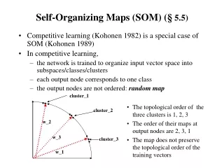
5. Kohonen self-organizing maps • SOM have been commonly used since their first description in a wide variety of problems • Classification • feature extraction • pattern recognition • other related applications. • An unsupervised classification algorithm from the artificial neural network paradigm.

6. Kohonen self-organizing maps(cont.) • After the learning stage each prototype represents a subset of the initial input set in which the inputs share some similar features. • Property • a vector quantization of the input space that respects the original distribution of the inputs. • prototypes are ordered according to their location in the input space. • does not hold for other standard vector quantization methods like competitive learning.

7. The double quantization method • The method described here aims to forecast long-term trends for a time series evolution • Base on the SOM algorithm and can be divided into two stages • the characterization：as the learning • the forecasting：as the use of a model in a generalization procedure.

8. Method description: characterization • Define the prediction of a vector • d is the size of the vector to be predicted • f is the data generating process • p is the number of past values that influence the future values • εt is a centred noise vector. • The past values are gathered in a p-dimensional vector called regressor. d P t-p+1 t+1 t+d t

9. Method description: characterization(cont.) • Inputs into regressors leads to n-p+1 vectors in a p-dimensional space, the resulting regressors are denoted: • p ≤ t ≤ n, p is the regressor size, n the number of value at our disposal in the time series. • x(t) is the original time series at our disposal with 1≤t ≤ n. • the subscript index denotes the first temporal value. • the superscript index denotes its last temporal value. t-p+1 t

10. Method description: characterization(cont.) • Deformation are created according: • Each is associated to one of the t-p+1 t-p+2 t t+1

11. Method description: characterization(cont.) • The SOM algorithm can then be applied to each one of these two spaces, quantizing both the original regressors and the deformations respectively. • All of the original space, n1 p-dimensional prototypes xi are obtained (1 ≤ i ≤n1), the clusters associated to xi are denoted ci. • All deformations in the deformation space results in n2 p-dimensional prototypes yj, 1 ≤ j ≤ n2, Similarly the associated clusters are denoted c’j.

12. Method description: characterization(cont.) • Define transition matrix f(ij): • The row fij for a fixed i and 1 ≤ j ≤ n2 is the conditional probability • belongs to c’j • belongs to ci.

13. Method description: forecasting • The prediction for time t+1 is obtain according to relation (3): • is the estimate of the true given by our time series prediction model. • look at row k in the transition matrix and randomly choose a deformation prototype among the according to the conditional probability distribution defined by fkj, 1 ≤ j ≤ n2 t-p+2 t+1

14. Method description: forecasting(cont.) • we extract the scalar prediction from the p-dimensional vector • to compute by (5) and tracting .We then do the same for • This ends the run of the algorithm to obtain a single simulation of the series at horizon h. • Monte-Carlo procedure is used to repeat many times the whole long-term simulation procedure at horizon h, as detailed above.

15. Method description: vector forecasting • is a vector defined as: • d is determined according to a priori knowledge about the series. • Example: when forecasting an electrical consumption, it could be advantageous to predict all hourly values for one day in a single step instead of predicting iteratively each value separately. t t+1 t+d

16. Method description: vector forecasting(cont.) • regressors of this kind of time series can be constructed: • The regressor is thus constructed as the concatenation of d-dimensional vectors from the past of the time series. • p: for the sake of simplicity, is supposed to be a multiple of d though this is not compulsory.

17. Method description: vector forecasting(cont.) • Deformation can be formed here according to: t-p+1 t-p+d+1 t t+d

18. Method description: vector forecasting(cont.) • Here again,the SOM algorithm can then be applied to each one of these two spaces, quantizing both the original regressors and the deformations respectively. • All of the original space, n1 prototypes are obtained (1 ≤ i ≤n1), the clusters associated to xi are denoted ci. • All deformations in the deformation space results in n2 prototypes , 1 ≤ j ≤ n2, Similarly the associated clusters are denoted c’j.

19. Method description: vector forecasting(cont.) • Define transition matrix as a vector generalisation of relation(4): • The row fij for a fixed i and 1 ≤ j ≤ n2 is the conditional probability • belongs to c’j • belongs to ci.

20. Method description: vector forecasting(cont.) • The simulation forecasting procedure can also be generalised: • consider the vector input for time t.The corresponding regressor is • find the corresponding prototype • choose a deformation prototypey among the according to the conditional distribution given by elements fkj of row k

21. Method description: vector forecasting(cont.) • The simulation forecasting procedure can also be generalised: • forecast as • extract the vectorfrom the d first columns of ^xttd tptdt1; • repeat until horizon h. • For this vector case ,Monte-Carlo procedure

22. Experimental result • This section is devoted to the application of the method on two times series. • Santa Fe A : scalar time series. • Polish electrical consumption form 1989 to 1996 : the prediction of a vector of 24 hourly values.

23. Experimental result(cont.) • Scalar forecasting : Santa Fe A • The completed data set contains 10,000 data. This set has been divided here as follows • the learning set contains 6000 data • the validation set 2000 data • test set 100 data • the regressors have been constructed according to • d = 1, p = 6 , value x(t+4) is omitted , and h = 100.

24. Experimental result(cont.) • Scalar forecasting : Santa Fe A • Kohonen strings of 1 up to 200 prototypes in each space have been used. • All the 40,000 possible models have been tested on the validation set. • The best model among them has 179 prototypes in the regressor space and 161 prototypes in the deformation space.

25. Experimental result(cont.) • Scalar forecasting : Santa Fe A

26. Experimental result(cont.) • Scalar forecasting : Santa Fe A

27. Experimental result(cont.) • Scalar forecasting : Santa Fe A

28. Experimental result(cont.) • Scalar forecasting : Santa Fe A

29. Experimental result(cont.) • Scalar forecasting : Santa Fe A

30. Experimental result(cont.) • Scalar forecasting : Santa Fe A

31. Experimental result(cont.) • Vector forecasting : the polish electrical consumption • The whole dataset contains about 72,000 hourly data

32. Experimental result(cont.) • Vector forecasting : the polish electrical consumption • our disposal 3000 data of dimension 24 • use 2000 of them for the learning • 800 for a simple validation • 200 for the test

33. Experimental result(cont.) • Vector forecasting : the polish electrical consumption • the optimal regressor is unknown, many different regressors were tried, using intuitive understanding of the process. The final regressor is: • p=5 data of dimension d=24 and Contain 2000+800 data • The forecasting obtained from this model is repeated 1000 times.

34. Experimental result(cont.) • Vector forecasting : the polish electrical consumption

35. Experimental result(cont.) • Vector forecasting : the polish electrical consumption

36. Experimental result(cont.) • Vector forecasting : the polish electrical consumption

37. Experimental result(cont.) • Vector forecasting : the polish electrical consumption

38. Conclusions • The use of SOMs makes it possible to apply the method both on scalar and vector time series and determine long-term trends.

39. My opinion • Advantage: Obtain long term trends • Apply • in the financial context • For the estimation of volatilities.