Time Series and Forecasting
130 likes | 343 Views
Time Series and Forecasting. Aggregate of supervisions of value Y, collected during some interval of time, name a Time series. It can be sequence of annual sales, quarterly income, a week's rate of exchange.

Time Series and Forecasting
E N D
Presentation Transcript
Time Series and Forecasting Aggregate of supervisions of value Y, collected during some interval of time, name a Time series. It can be sequence of annual sales, quarterly income, a week's rate of exchange. The basic standards for such class of tasks - information must be collected for large period and necessarily for the equal intervals of time. It means that information collect each quarter and in all of table of basic data they are set every quarter. Or information collect every year, then a time interval is equal to the year, or hour, or month. It is one constant interval always. • Decomposition- one of methods of analysis of Time series. He carries out the selection of making factors of Time series. He is used and for short-term and long-term prognoses. • Models, built from data, to characterizing one object for the row of successive moments (periods), are named the models of Time series. A Time series is an aggregate of values of some index for a few successive moments or periods. Every level of temporal row is formed from: • trend (Т), • cyclic (С), • seasonal (S) , • casual (I) component.
Trend - long-term component, describing influencing of time row the effect of which tells gradually. • Cyclic component describes the prolonged periods of getting up and slump. • Seasonal component describes repetition of processes in time. • The determined components describe a time row not fully, it is necessary to take into account a chance. It is irregular components. They are conditioned influence of great number of insignificant factors which together can make the serious affecting on result. Models in which a time row is presented as a sum of component are additive models. If use an increase component, it is multiplicative models of temporal row. An additive model looks like Y = Т + S + I+C; multiplicative model: Y=Т S IC.
On the screen you see the file of Excel with information about the results of sales. Alongside there is a chart. On an axis Х the sequence number of information is shown, on an axis at are volumes of sales. Information fixed every year. Open the file of Excel and carry information from the package of Excel in the package of Statistica.
Open the module Time Series and Forecasting. Open a menu Analysis /Startup panel.
Number of backups per variable – a maximal number of variables is in a work area. Task a variable. ARIMA & autocorrelation functions- model of autoregression and sliding middle. Interrupted time series analysis – analysis of the interrupted temporal rows. Exponential smoothing & forecasting –exponential smoothing out and prognostication Distributed lags analysis –regressive model of 2th temporal rows Replace missing data – what to replace the skipped information: Overall mean –general middle Interpolation from adjacent pointsinterpolation on the nearest points Mean of N adjacent points –to replace average on a few points Median of N adjacent points - to replace a median on a few points Predicted values from linear trend regression – prognosis on the basis of trend.
Choose a point Arima. You will see a starting window for prognostication Its parameters: Estimate constant-Whether it is needed to enter a constant additionally. Seasonal lag - Set values P-Seasonal and Q-Seasonal. If series are long (365 days in a year), it is recommended to set a maximum likelihood method. Autoregressive parameters. p -parameter of autoregressive. P–seasonal parameter of autoregressive. q–parameter sliding middle. Q - parameter sliding middle.
Models of Autoregressionand model with distributed lag Lag variables- temporal rows of variables, shift on one or more than moments of time. Models, containing not only current but also the lag values of variables are named models with distributed lag. For determination of composition of components (structures of temporal row) in the model of temporal row build a autocorrelation model. This model talks that if in some moment of time of t there is a change an independent variable X, this change will influence on variable of Y values during the next moments of time of L (lag). Autocorrelationis correlation connection between the successive levels of the same row of dynamics (moved on the certain interval of time of L -lag). That, autocorrelation is connection between a row: x1, x2, ... xn- l and rowx1+l, x2+l, ...,xn, where L- positive integer. Autocorrelation can be measured the coefficient of autocorrelation. You can expect it in Excel by the function of КОРРЕЛ.
At first it is necessary to create arrays with a shift on a 1 line down. For example, in the moment of time t array was in limits from 4 to 42 lines. The array of Yt-1 is moved on a 1 line downward and is from 4 lines to 42. Superfluous lines at a change are deleted. There must be an equallyamount of elements at arrays. Such picture must turn out for you: Correlation for the first array is considered on a formula =КОРРЕЛ(C4:C42;E4:E42)
You will define correlations for 7 periods of time. Such numbers must appear for you: Find the maximal value of correlation. In our table it is equal to 0.70809, it is a shift on 4. Value 4 enter in a window, shown on a slide6, seasonal lag. Set in the model of p=1, q=1, P=1,Q=1. Number 1 determines the type of dependence. If parameters are equal to 1, search linear equationfor a prognosis. If parameters are equal to 2, dependence has the appearance of parabola. If you consider that season plays a most role, set for the parameters of P and Q values, equal 3 or 4, and leave autoregression equal 1.
Press the button OK for the beginning of calculations. After a report, that a process converged, you would get the window of results: In the window of Numberofcases input, what period a prognosis is built on, for example, in our file value 4 means that on a year. We examined quarter information. Press the button Forecasting and copy information in Excel, add it on a chart.
The button PlotSeries builds a chart, a red color is show a prognosis, blue - observed data, green is a prognosis for situations successful and vice versa.
Window of the forecast information Error Estimation of model exactness
Sequence of executions: 1. To build a chart in Excel, setting aside on an ax Х - temporal the component of t, to on Y are volumes of sales. 2. To estimate the tendencies of sales by sight. 3. To carry information in the package of Statistica. To open StartUpPanel, set a variable for an analysis. 4. To choose the method of Arima. 5. In Excel to define the size of lag. For this purpose by the function of КОРРЕЛ to define its maximal value and number of lag which he corresponds. 6. In the window of parameters to set the values of parameters for a start p=1 , q=1, P=1,Q=1. Input seasonal lag, expected on a previous step. After completion of calculations to estimate the sizes of Residals(button ParameterEstimations). To fix the size of Residals. 7. To change the sizes of parameters, for example, p=2, q=2, P=1,Q=1. To estimate the sizes of residals (button ParameterEstimations) . Compare with got on a previous step in size Residals. To leave a less value. 8. To change parameters until residals will decrease. 9. After it to press the button Forecasting and Plotsofresiduals . To copy forecasting information, carry them in Excel, to add to the chart.