Download

1 / 64
650 likes | 758 Views
Learn effective strategies for the final exam in Image Processing course. Understand image classification, processing tasks, and the importance of synthesizing information. Key topics include digital image analysis and image slicing.

E N D
Classification & Analysis of Digital MSS Data Lecture 8 Summer Session 09 August 2011
Tips for the Final Exam • Make sure your answers clear, without convoluted language. • Read questions carefully – are you answering the entire question? • Be thorough! • Synthesize material you have learned in this class. • Think about applications of remote sensing science – tie in your lab experiences with what you have learned from the book/lecture. • Likely format: • 14 multiple choice - 2 points each = 28 • 10 short answer – 4 points (9) or 6 points (1) each = 42 • You will have choices for most – 1A or 1B, 2A or 2B, etc. • 2 or 3 essay questions – total of 50 points • You will probably have choices here, too. • Longer, more challenging, more comprehensive. • Extra Credit Assignment Lab worth 3%, due 18 August before final exam
Goals for image processing • Identify • Features, single or multiple characteristics, areas of change, etc. • Quantify • Spatial extent of features • Magnitude of features (levels; e.g. fire severity, or extent of burn) • Analyze • Derive meaningful information
Image Processing – 3 Primary Tasks • Identify and map a specific feature of interest on the imagery • e.g. identify deforested areas • Create a map with multiple categories or levels • e.g. create a land cover map • Create maps that represent different levels of a surface/atmosphere characteristic • estimate net primary production in oceanic regions • A map of different levels of the same characteristic • e.g. percent tree cover – 0-100%
Single Characteristic Multiple Categories Different levels of a single characteristic
Image Classification The process of automatically dividing all pixels within a digital remote sensing image into: • Land or surface-cover categories • Information themes or quantification of specific surface characteristics
From: http://www.fes.uwaterloo.ca/crs/geog376.f2001/ ImageAnalysis/ImageAnalysis.html#ImageProcessingSteps
1: Evergreen Needleleaf Forests; 2: Evergreen Broadleaf Forests; 3: Deciduous Needleleaf Forests; 4: Deciduous Broadleaf Forests; 5: Mixed Forests; 6: Woodlands; 7: Wooded Grasslands/Shrubs; 8: Closed Bushlands or Shrublands; 9: Open Shrublands; 10: Grasses; 11: Croplands; 12: Bare; 13: Mosses and Lichens http://www.geog.umd.edu/landcover/8km-map.html
Cropland Probability – 0-100% Pittman et al. (2010)
SeaWiFS (Sea-viewing Wide Field-of-view Sensor) image classification: chlorophyll concentration in the Gulf of Mexico
Image Slicing and Thresholding • Thresholding of digital values • i.e. % reflectace or DN • Thresholding of transformed values • e.g. NDVI, NBR, etc.
Image classification based on average data values in a single channel is a risky undertaking
This block represents a single land cover type 14 15 17 15 Average = 14.75 Range = 11 - 18 16 13 18 14 16 15 13 15 17 15 11 12 Most land surfaces have a range of values, not a single value
Lillesand and Kiefer Figure 7-46 Unless the average values are very far apart, a significant number of mis-classified pixels will be produced as a result of a single band thresholding
Lillesand and Kiefer Figure 7-11 When the differences between features of interest are high, it is possible to use a simple threshold to discriminate between the features (water vs. land surface)
Water The range in digital values for these two surfaces do not overlap, so you can use a level slice to classify your image into two categories > 40 = Land < 40 = water Land Lillesand and Kiefer Figure 7-11
Two-step level slicing or thresholding Step 1 – Estimate the range of values of a given surface characteristic on a single band e.g. vegetation on Landsat 7 ETM+ Band 4 Step 2 – create discrete levels of the characteristic “slice” up the histogram
Example of 2-step level slice With AVHRR data, greenness can be estimated from the Normalized Difference Vegetation Index (NDVI) Greenness = (Near IR – Red) (Near IR + Red)
Image Classification Because we have seen the limitations of density slicing, or single-band classifications… Let’s look at how exactly multiple bands of information are combined to perform a multiband classification…
Challenge in remote sensing – how does one capture the information content that is available in the different channels of the digital image?
If you find this interesting, read up on “the tasseled cap transformation” Lillesand and Kiefer Figure 7-39
Image Classification The process of automatically dividing all pixels within a digital remote sensing image into discrete categories • Supervised vs. unsupervised
Supervised vs. Unsupervised Classification • Supervised classification – a procedure where the analyst guides or supervises the classification process by specifying numerical descriptors of the land cover types of interest • Unsupervised classification – the computer is allowed to aggregate groups of pixels into like clusters based upon different classification algorithms
Training Areas and Supervised Classification • Specified by the analyst to represent the land cover categories of interest • Used to compile a numerical “interpretation key” that describes the spectral attributes of the areas of interest • Each pixel in the scene is compared to the training areas, and then assigned to one of the categories
Multiband Classification Approaches • Minimum distance classifiers* • Parallelepiped classifiers* • Maximum likelihood classifiers* • Decision trees* • Neural networks *covered in class (know for exam)
Minimum Distance Classifiers Step 1 – calculate the average value for each training area in each band f f + f f f c c c c + c
Minimum Distance Classifiers Step 2 – for each unclassified pixel, calculate the distance to the average for each training area The unclassified pixel is place in the group to which it is closest f f + f f f * c c c c + c * - Unclassified pixel
Minimum Distance Classifiers Lillesand and Kiefer Figure 7-40
Advantages/Disadvantages of Minimum Distance Classifiers • Advantages • Simple and computationally efficient • Disadvantages – • Does not factor in the fact that some categories have a large variance • e.g. pixel #2 on last slide ended up on sand, but could have been urban!
Parallelepiped Classifiers Step 1 – define the range of values in each training area and use these ranges to construct an n-dimensional box (a parallelepiped) around each class f f f f f c c c c c
a pixel falls into a category if it falls within the N-dimensional box, otherwise it is unclassified • a problem with the PP is that there can be overlap between categories Lillesand and Kiefer Figure 7-41
Fix the overlappinjg regions with a parallelepiped classifier with a stepped decision region boundary Lillesand and Kiefer Figure 7-41
Maximum likelihood classifiers • Based on a probability function derived from a statistical distribution of reflectance values
Plots of DN values fit create a histogram which usually fit a certain statistical distribution Lillesand and Kiefer Figure 7-46
There are statistical functions or equations which describe the distribution of data
Lillesand and Kiefer Figure 7-43 a 3-dimensional normal curve fit to the data values from an example of Digital values from the two channels of the Landsat scene
Steps for maximum likelihood classifier • Determine the n-dimensional curve for a particular feature • Fit it to normal distribution • Use statistical algorithms to describe them • Define the levels of probability acceptable for classification of a given pixel
Maximum likelihood classifiers the equal probability contours that were constructed around the different training areas are used to classify the images Max likelihood classifier selects the category with highest probability for a pixel Lillesand and Kiefer Figure 7-44
Unsupervised classification • Lack of a priori information on what types of land or vegetation cover types exist within a region • BUT: it may be difficult to interpret the computer generated classes
Unsupervised Classification Allow the computer to identify clusters based on different classification procedures Lillesand and Kiefer Figure 7-51
Hybrid Classification Approach • Perform an unsupervised classification to create a number of land cover categories within the area of interest • Carry out field surveys to identify the land cover type represented by different unsupervised clusters • Use a supervised approach to combine unsupervised clusters into similar land cover categories
Sources of Uncertainty in Image Classification • Non-representative training areas • High variability in the spectral signatures for a land cover class • Mixed land cover within the pixel area
Mixed pixels In many cases, the IFOV of a sensor will include multiple land cover categories – e.g., a mixed pixel Mixed pixels contribute to classification errors
Question – How do different algorithms treat mixed pixels? In some cases, mixed pixels are close enough to a specific category, which leads to misclassifications d d d f m d f f f d f m m m c m c c c c