Understanding Bi-linear and Bi-cubic Interpolation in Digital Images
This document explores the concepts of bi-linear and bi-cubic interpolation techniques used in digital image processing. Using specific examples, it demonstrates how to calculate values at non-integer coordinates (e.g., G(3.6, 2) and G(3.6, 2.3)) based on given integer values. The calculations involve horizontal and vertical positions, grey levels, and the development of cubic curves to derive new pixel values smoothly. By following the mathematical processes outlined, readers will gain insights into image interpolation's practical application in enhancing image quality.

Understanding Bi-linear and Bi-cubic Interpolation in Digital Images
E N D
Presentation Transcript
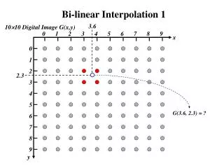
Bi-linear Interpolation 1 1010 Digital Image G(x,y) 3.6 0 1 2 3 4 5 6 7 8 9 x 0 1 2 2.3 3 4 5 G(3.6, 2.3) = ? 6 7 8 9 y
Bi-linear interpolation 2 G(3.6,2)=? G(3,2)=58 G(4,2)=150 Calculate G(3.6,2) by using values of G(3,2) and G(4,2): G(3.6,2.3)=? Grey level 255 150 113.2 58 Horizontal position 1 2 3 4 0 3.6 G(3.6,3)=? G(3,3)=137 G(4,3)=26 G(3.6,2) = (1fx)G(3,2) + fxG(4,2), Wherefxis 0.6 (fraction part of 3.6) And G(3,2)=58, G(4,2)=150, so G(3.6,2) = 113.2 In the same way G(3.6,3) = (1fx)G(3,3) + fxG(4,3) = (1-0.6)137 + 0.626 = 70.4
Bi-linear interpolation 3 G(3.6,2)=113.2 G(3,2)=58 G(4,2)=150 Calculate G(3.6,2.3) by using values of G(3.6,2) and G(3.6,3): G(3.6,2.3)=? Grey level 255 113.2 100.36 70.4 Vertical position G(3.6,3)=70.4 G(3,3)=137 G(4,3)=26 1 2 3 4 0 2.3 G(3.6,2.3) = (1fy)G(3.6,2) + fyG(3.6,3), Wherefy is 0.3 (fraction part of 2.3) And G(3.6,2)=113.2, G(3.6,3)=70.4, so G(3.6,2.3) = 100.36
Bi-cubic Interpolation 1 1010 Digital Image G(x,y) 3.6 0 1 2 3 4 5 6 7 8 9 x 0 1 2 2.3 3 4 5 G(3.6, 2.3) = ? 6 7 8 9 y
Bi-cubic interpolation 2 G(2,1)=34 G(3,1)=102 G(4,1)=10 G(5,1)=86 G(3.6,1)=? G(3.6,2)=? G(5,2)=205 G(2,2)=95 G(3,2)=58 G(4,2)=150 G(3.6,2.3)=? G(2,3)=220 G(3,3)=137 G(4,3)=26 G(5,3)=134 G(3.6,3)=? G(2,4)=78 G(3,4)=186 G(4,4)=18 G(5,4)=214 G(3.6,4)=?
Bi-cubic interpolation 3 Calculate G(3.6,1) by using values of G(2,1), G(3,1), G(4,1) and G(5,1): Cubic curve: f(t) = a3 · t3 + a2 · t2 + a1 ·t + a0 f(2) = 34 f(3) = 102 f(4) = 10 f(5) = 86 Solve the above linear functions, we can decide the values of a3 ,a2 ,a1 and a0. Then f(3.6) can be calculated. Grey level 255 f 102 86 51.14 34 10 Horizontal position 0 4 2 3 5 1 3.6 Result: G(3.6, 1) = 51.14 Using the same strategy, we can calculate the values of G(3.6, 2) = 113.25, G(3.6, 3) = 83.37, G(3.6, 4) = 95.36
Bi-cubic interpolation 4 G(2,1)=34 G(3,1)=102 G(4,1)=10 G(5,1)=86 G(3.6,1)=51.14 G(3.6,2)=113.25 G(5,2)=205 G(2,2)=95 G(3,2)=58 G(4,2)=150 G(3.6,2.3)=? G(2,3)=220 G(3,3)=137 G(4,3)=26 G(5,3)=134 G(3.6,3)=83.37 G(2,4)=78 G(3,4)=186 G(4,4)=18 G(5,4)=214 G(3.6,4)=95.36
Bi-cubic interpolation 5 Calculate G(3.6,2.3) by using values of G(3.6,1), G(3.6,2), G(3.6,3) and G(3.6,4): From the previous slide we know: G(3.6, 1) = 51.14 ,G(3.6, 2) = 113.25, G(3.6, 3) = 83.37, G(3.6, 4) = 95.36. Cubic curve: f(t) = a3 · t3 + a2 · t2 + a1 ·t + a0 f(2) = 51.14 f(3) = 113.25 f(4) = 83.37 f(5) = 95.36 Solve the above linear functions, we can decide the values of a3 ,a2 ,a1 and a0. Then f(2.3) can be calculated. Grey level 255 f(2.3) = 99.21 f 113.25 95.36 83.37 51.14 Vertical position 0 4 2 3 5 1 2.3 Result: G(3.6, 2.3) = 99.21