Understanding Data Points and Interpolation in MATLAB
This guide explains the concepts of data points and interpolation using MATLAB. Data points represent values at specific horizontal positions, while interpolation helps estimate values at grid lines that do not correspond to actual data points. We discuss various interpolation methods, such as Nearest Neighbor, and emphasize the need for well-placed grid lines to improve accuracy. Furthermore, we demonstrate how to organize data in matrices for MATLAB plotting and detail code writing practices for effective interpolation.


Understanding Data Points and Interpolation in MATLAB
E N D
Presentation Transcript
Interpolation Data Point -A data point is a value at some position. Consider position along the horizontal axis for now. Then the picture below shows four data points, each value shown as a height of an x at its horizontal position. x x x x
Interpolation Grid Line -An imaginary vertical line at some position which may not correspond to a data point's position. A value is associated with a grid line – we use circles in the figure to illustrate. ⊙ ⊙ x x ⊙ ⊙ ⊙ ⊙ ⊙ ⊙ ⊙ x ⊙ ⊙ ⊙ ⊙ x ⊙ ⊙
Interpolation A graph – Given a collection of grid lines, with values, Matlab will fill the spaces between grid lines with straight lines connecting the dots representing values. For example, see below: ⊙ ⊙ x x ⊙ ⊙ ⊙ ⊙ ⊙ ⊙ ⊙ x ⊙ ⊙ ⊙ ⊙ x ⊙ ⊙
Interpolation This example – The line below does a bad job of representing the four data points: it is jumpy and it does not even come close to the data points. We need a way to find grid line values that allow Matlab to better approximate the data. ⊙ ⊙ x x ⊙ ⊙ ⊙ ⊙ ⊙ ⊙ ⊙ x ⊙ ⊙ ⊙ ⊙ x ⊙ ⊙
Interpolation Nearest Neighbor – The simplest, but hardly the best, way to get grid line values is to use the value of the nearest data point. For example, consider this grid line: x x x x
Interpolation Nearest Neighbor – The simplest, but hardly the best, way to get grid line values is to use the value of the nearest data point. Look for the nearest data point to the grid line: 0.35 x 0.83 x x x 0.21 2.05 0 0.2 0.4 0.6 0.8 1.0 1.2 1.4 1.6 1.8 2.0 2.2 2.4 2.6 2.8 3.0 ...
Interpolation Nearest Neighbor – The simplest, but hardly the best, way to get grid line values is to use the value of the nearest data point. The closest data point is the 2nd from left – the value of the grid line is the value of that point: x x ⊙ x x
Interpolation Nearest Neighbor – The simplest, but hardly the best, way to get grid line values is to use the value of the nearest data point. Continue for all the grid points. ⊙ ⊙ ⊙ ⊙ x x ⊙ ⊙ ⊙ ⊙ ⊙ ⊙ ⊙ x x ⊙ ⊙ ⊙ ⊙
Interpolation Nearest Neighbor – The simplest, but hardly the best, way to get grid line values is to use the value of the nearest data point. Using plot(...) Matlab shows this: x x x x
Interpolation Variables – 1: The data will have to reside somewhere. Matlab likes matrices so put the data in a two dimensional array: 1st column is the x position, 2nd column holds the data values, the number of rows is the number of data pts. Call the matrix dpts. x x dpts(1,1) x dpts(1,2) x 0
Interpolation Variables – 1: The data will have to reside somewhere. Matlab likes matrices so put the data in a two dimensional array: 1st column is the x position, 2nd column holds the data values, the number of rows is the number of data pts. Call the matrix dpts. x x x x dpts(2,1) dpts(2,2) 0
Interpolation Variables – 1: The data will have to reside somewhere. Matlab likes matrices so put the data in a two dimensional array: 1st column is the x position, 2nd column holds the data values, the number of rows is the number of data pts. Call the matrix dpts. x x x x dpts(3,1) dpts(3,2) 0
Interpolation Variables – 2: The position and value of grid lines will reside somewhere. Since we will use plot(x,y) to plot the result, it is convenient to define vectors x and y to mean position and value, respectively. Since we can choose the grid line positions, we can set that vector right away. X = 0:0.2:10; x x x x 0 0.2 0.4 0.6 0.8 1.0 1.2 1.4 1.6 1.8 2.0 2.2 2.4 2.6 2.8 3.0 ...
Interpolation Variables – 2: The position and value of grid lines will reside somewhere. Since we will use plot(x,y) to plot the result, it is convenient to define vectors x and y to mean position and value, respectively. Since we can choose the grid line positions, we can set that vector right away. X = 0:0.2:10; and the length of the y vector must match this so we can do y = zeros(length(x)); x x x x 0 0.2 0.4 0.6 0.8 1.0 1.2 1.4 1.6 1.8 2.0 2.2 2.4 2.6 2.8 3.0 ...
Interpolation Writing the code – For each grid line we need to determine which data point is nearest, then set the value of the grid line to the value of that data point. x x x x 0 0.2 0.4 0.6 0.8 1.0 1.2 1.4 1.6 1.8 2.0 2.2 2.4 2.6 2.8 3.0 ...
Interpolation Writing the code – For each grid line we need to determine which data point is nearest, then set the value of the grid line to the value of that data point. Start off with a simpler problem: find data point nearest to some grid line x x x x 0 0.2 0.4 0.6 0.8 1.0 1.2 1.4 1.6 1.8 2.0 2.2 2.4 2.6 2.8 3.0 ...
Interpolation Ask questions – To find distances from grid line to a data point I need to known the position of the grid line and the position of the data point. x x x x 0 0.2 0.4 0.6 0.8 1.0 1.2 1.4 1.6 1.8 2.0 2.2 2.4 2.6 2.8 3.0 ...
Interpolation Ask questions – To find distances from grid line to a data point I need to known the position of the grid line and the position of the data point. We said the grid line position is in a vector called x. But to access an element of x I need to provide an index (i.e. x(i)). For now, we use this and figure out how to get i later. x x x x x(i) 0 0.2 0.4 0.6 0.8 1.0 1.2 1.4 1.6 1.8 2.0 2.2 2.4 2.6 2.8 3.0 ...
Interpolation Ask questions – To find distances from grid line to a data point I need to known the position of the grid line and the position of the data point. Consider the position of the 1st data point – we said it is dpts(1,1). x x dpts(1,1) x x x(i) 0 0.2 0.4 0.6 0.8 1.0 1.2 1.4 1.6 1.8 2.0 2.2 2.4 2.6 2.8 3.0 ...
Interpolation Ask questions – To find distances from grid line to a data point I need to known the position of the grid line and the position of the data point. Now to find the distance between grid line and data point 1 I can use abs(x(i)-dpts(1,1)). abs(x(i)-dpts(1,1)) x x dpts(1,1) x x x(i) 0 0.2 0.4 0.6 0.8 1.0 1.2 1.4 1.6 1.8 2.0 2.2 2.4 2.6 2.8 3.0 ...
Interpolation Ask questions – To find distances from grid line to a data point I need to known the position of the grid line and the position of the data point. But I need to do this for all the data points. Moreover, I need to compare results and pick the data point for which abs(...) is lowest. abs(x(i)-dpts(1,1)) abs(x(i)-dpts(3,1)) x x abs(x(i)-dpts(2,1)) x x abs(x(i)-dpts(4,1)) 0 0.2 0.4 0.6 0.8 1.0 1.2 1.4 1.6 1.8 2.0 2.2 2.4 2.6 2.8 3.0 ...
Interpolation Write code – I can use a for loop to compute all the abs(...) terms on each interation I can compare another data point. But to write the for loop I need to know the number of points. abs(x(i)-dpts(1,1)) abs(x(i)-dpts(3,1)) x x abs(x(i)-dpts(2,1)) x x abs(x(i)-dpts(4,1)) 0 0.2 0.4 0.6 0.8 1.0 1.2 1.4 1.6 1.8 2.0 2.2 2.4 2.6 2.8 3.0 ...
Interpolation Write code – I will figure out how to get it later. For now I will suppose a variable called npts holds that number. So I write: for j=1:npts abs(x(i) – dpts(j,1)); end x x x x 0 0.2 0.4 0.6 0.8 1.0 1.2 1.4 1.6 1.8 2.0 2.2 2.4 2.6 2.8 3.0 ...
Interpolation Write code – This is no good – I will save results (dss) and compare with a previous best (dsx): for j=1:npts dss = abs(x(i) – dpts(j,1)); if dss < dsx dsx = dss; end end x x x x 0 0.2 0.4 0.6 0.8 1.0 1.2 1.4 1.6 1.8 2.0 2.2 2.4 2.6 2.8 3.0 ...
Interpolation Write code – Still no good – I will also save the index (bst) of the current nearest data point: for j=1:npts dss = abs(x(i) – dpts(j,1)); if dss < dsx dsx = dss; bst = j; end end x x x x 0 0.2 0.4 0.6 0.8 1.0 1.2 1.4 1.6 1.8 2.0 2.2 2.4 2.6 2.8 3.0 ...
Interpolation Write code – Hold the phone – dsx has no value when j=1 so I pull the first abs() out of the loop and start with j=2 dsx = abs(x(i) – dpts(1,1)); bst = 1; for j=2:npts dss = abs(x(i) – dpts(j,1)); if dss < dsx dsx = dss; bst = j; end end 0 0.2 0.4 0.6 0.8 1.0 1.2 1.4 1.6 1.8 2.0 2.2 2.4 2.6 2.8 3.0 ...
Interpolation Write code – Finally, I need to set the value of the ith grid line (this is y(i)) dsx = abs(x(i) – dpts(1,1)); bst = 1; for j=2:npts dss = abs(x(i) – dpts(j,1)); if dss < dsx dsx = dss; bst = j; end end y(i) = dpts(bst,2); 0 0.2 0.4 0.6 0.8 1.0 1.2 1.4 1.6 1.8 2.0 2.2 2.4 2.6 2.8 3.0 ...
Interpolation Write code – Now I have to repeat this for all the grid lines for i=1:length(y) dsx = abs(x(i) – dpts(1,1)); bst = 1; for j=2:npts dss = abs(x(i) – dpts(j,1)); if dss < dsx dsx = dss; bst = j; end end y(i) = dpts(bst,2); end 0 0.2 0.4 0.6 0.8 1.0 1.2 1.4 1.6 1.8 2.0 2.2 2.4 2.6 2.8 3.0 ...
Interpolation Write code – Let's add in what we have from before x=0:0.2:10; y=zeros(length(x)); for i=1:length(y) dsx = abs(x(i) – dpts(1,1)); bst = 1; for j=2:npts dss = abs(x(i) – dpts(j,1)); if dss < dsx dsx = dss; bst = j; end end y(i) = dpts(bst,2); end plot(x,y); 0 0.2 0.4 0.6 0.8 1.0 1.2 1.4 1.6 1.8 2.0 2.2 2.4 2.6 2.8 3.0 ...
Interpolation Write code – The only things missing are the data points and setting npts. x=0:0.2:10; y=zeros(length(x)); for i=1:length(y) dsx = abs(x(i) – dpts(1,1)); bst = 1; for j=2:npts dss = abs(x(i) – dpts(j,1)); if dss < dsx dsx = dss; bst = j; end end y(i) = dpts(bst,2); end plot(x,y); 0 0.2 0.4 0.6 0.8 1.0 1.2 1.4 1.6 1.8 2.0 2.2 2.4 2.6 2.8 3.0 ...
Interpolation Write code – Read the data from a file – suppose file's name is one.dat and it begins with a line containing the number of data points and each line thereafter is a data point with position followed by value (two numbers/line). Open the file and read the number of data points. fid = fopen('one.dat','r'); if fid < 1 error('No such file'); end npts = fscanf(fid,'%d',1); % number points
Interpolation Write code – Read the data from a file – suppose file's name is one.dat and it begins with a line containing the number of data points and each line thereafter is a data point with position followed by value (two numbers/line). Create the dpts matrix so we can store the data from file fid = fopen('one.dat','r'); if fid < 1 error('No such file'); end npts = fscanf(fid,'%d',1); % number points dpts = zeros(npts,2);
Interpolation Write code – Read the data from a file – suppose file's name is one.dat and it begins with a line containing the number of data points and each line thereafter is a data point with position followed by value (two numbers/line). Now store the data points fid = fopen('one.dat','r'); if fid < 1 error('No such file'); end npts = fscanf(fid,'%d',1); % number points dpts = zeros(npts,2); for i=1:npts dpts(i,:) = fscanf(fid,'%f',2); end
Interpolation Write code – Read the data from a file – suppose file's name is one.dat and it begins with a line containing the number of data points and each line thereafter is a data point with position followed by value (two numbers/line). Close the file. Merge this part with the previous part. fid = fopen('one.dat','r'); if fid < 1 error('No such file'); end npts = fscanf(fid,'%d',1); % number points dpts = zeros(npts,2); for i=1:npts dpts(i,:) = fscanf(fid,'%f',2); end fclose(fid);
Interpolation 2D – Each line of the file has 2 coordinates plus a value. Grid lines occur at mesh points – each with x,y coordinates. Let x be an x position vector as before. Establish a y vector for the y position of a grid line. Expand dpts so dpts(k,2) is the y position of the data point and dpts(k,3) is the value. Then, distance from grid line to data point is sqrt((x(i)-dpts(k,1))^2+(y(j)-dpts(k,2))^2) which computes distance between the (i,j) grid line and the kth data point. Use vector v to hold interpolated values and z to hold grid line values. Then the inner loop ends w/ z(i,j) = dpts(bst,3); and the output loop becomes two loops (i and j).
Interpolation 1D - Inverse Distance Squared d1 f(x1 ) x x f(x3 ) d3 x f(x2 ) x d2 f(x4 ) d4 xp
Interpolation 1D - Inverse Distance Squared d1 f(x1 ) x x f(x3 ) d3 x f(x2 ) x d2 f(x4 ) d4 xp f(xp ) = (f(x1 )/d12 + f(x2 )/d22 + f(x3 )/d32 + f(x4 )/d42)/(1/d12 +1/ d22 +1/ d32 +1/ d42)
Interpolation 1D - Inverse Distance Squared d1 f(x1 ) x x f(x3 ) d3 x f(x2 ) x d2 f(x4 ) d4 xp Use 1/(+d2) instead of 1/d2 to prevent blowup!