Linear Interpolation

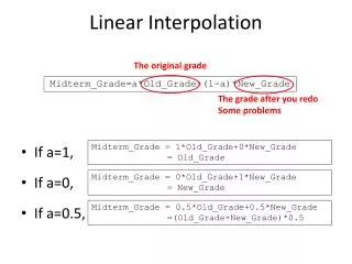
Linear Interpolation The original grade Midterm_Grade=a*Old_Grade+(1-a)*New_Grade The grade after you redo Some problems Midterm_Grade = 1*Old_Grade+0*New_Grade = Old_Grade • If a=1, • If a=0, • If a=0.5, Midterm_Grade = 0*Old_Grade+1*New_Grade = New_Grade Midterm_Grade = 0.5*Old_Grade+0.5*New_Grade =(Old_Grade+New_Grade)*0.5

Linear Interpolation • Now if you change the grade into two vertices: Va=a*V1+(1-a)*V0 V1 a>1 V0.5 a=1 a=0.75 V0 a=0.5 a=0.25 a=0 a<0 This is how we define a line, a line segment, or a ray.

Linear Interpolation • Now if know V1, V2, and V, how do you know a instead? • We know: V=a*V1+(1-a)*V0 V-V0=a*(V1-V0) a=|V-V0|/|V1-V0| V1 |V-V0| V a V0 |V1-V0|

Linear Interpolation • Now if you have two values C0 and C1 (color, depth, texture coordinates…) at V0 and V1, how to get the value Ca at V: a=|V-V0|/|V1-V0| Ca=a*C1+(1-a)*C0 V1 |V-V0| C1 V a Ca??? V0 |V1-V0| C0

Midterm Grading Formula Midterm_Grade=(a*Old_Grade+(1-a)*New_Grade)b a: Interpolation coefficient b: Curve coefficient • Option 1: No new grade, just curve it. (a=1) • Option 2: Redo two questions, take the average and curve it. (a=0.5) • Option 3: Redo two questions, take the average but no curve. (a=0.5, b=1) • Option 4: Redo all questions, take the average but no curve. (a=0.5, b=1)

Midterm Grading Formula • Redo two questions • Pro: less work for you (and for me) • Con: depends on the choice of questions, not very fair for some people: • A: 3+3+3+3+3=15 (old); 3+5+5+3+3=19 (new). • B: 5+0+0+5+5=15 (old); 5+5+5+5+5=25 (new). • Redo all questions • Con: more work • Pro: you get the second chance to learn; and it is relatively fair

Midterm Grading Formula • Details: • Return the graded old exam package to you now (on Wednesday). So you know which answer is wrong and which is right. • Only the old grade, but not the exam package. You know your overall performance, but don’t know which answer is wrong exactly. • After you submit your new answers, you will get the graded old exam package.

Homogenous Space Vs. 3D Space A point in the 3D Space A point in the homogenous Space (4D) A point in the 3D Space A point in the homogenous Space

Homogenous Space Vs. 3D Space What if w is not 1? Scale it by 1/w! A point in the 3D Space A point in the homogenous Space

Projection and Transformation A point in the 3D Space A point in the homogenous Space (4D) Multiply it by your matrix Your solution in 3D! Your result in the homogenous Space (4D)

Projection and Transformation Transformation won’t change w. w is always 1. 2D image location Depth Value (Z value) Projection changes w!

Transformation One way to understand the transformation: Its changed position in the absolute space A point in an absolute space

Transformation Another way to understand the transformation: The same point, but in a new space A point in one space

Transformation A point in the local space (or called the model space) A point in the eye space (or called the camera space) A point in the local space (or called the model space) A point in the eye space (or called the camera space)

Transformation (eye space -> eye space) glLoadIdentity(); glRotatef(…); glTranslatef(…); glScalef(…); glBegin(GL_POINTS); glVertex3fv(v); glEnd(); (space No. 1 -> eye space) (space No. 2 -> eye space) (space No. 3 -> eye space) (space No. 3 -> eye space)

Transformation The matrix not only transforms a vertex from the local space into the eye space, it also tells us how the local space looks like in the eye space: The local X axis The local Z axis The local Y axis The local Origin

Transformation Eye space glLoadIdentity(); //Camera motions (also as transformation) //Do more transformations glBegin(GL_POINTS); glVertex3fv(v); glEnd(); World space Local space OpenGL only has the modelview matrix, which really contains two steps: viewing and modeling.

Shading • Now you did projection, you have polygons in 2D. • You do rasterization, so you have scanlines. Each line have two endpoints and you have a lot of pixels between them. • Suppose you have a function f(x) that can give you a value at any point, how do you use it to get a value for each pixel? f(Vs) f(V1) f(V0) V0 V1 Vs Phong Shading

Shading • Now you did projection, you have polygons in 2D. • You do rasterization, so you have scanlines. Each line have two endpoints and you have a lot of pixels between them. • Suppose you have a function f(x) that can give you a value at any point, how do you use it to get a value for each pixel? f(V0) f(V0) f(V0) f(V0) f(V0) f(V0) V0 V1 Vs Flat Shading

Shading • Now you did projection, you have polygons in 2D. • You do rasterization, so you have scanlines. Each line have two endpoints and you have a lot of pixels between them. • Suppose you have a function f(x) that can give you a value at any point, how do you use it to get a value for each pixel? sf(V1)+(1-s)f(V0) f(V1) f(V0) V0 V1 Vs Gouroud Shading

Geometric Modeling

Basic GLUT Shapes • Spheres • Cones • Cubes glutWireSphere(radius, slices, stacks) glutSolidSphere(radius, slices, stacks) glutWireCone(radius, height, slices, stacks) glutSolidCone(radius, height, slices, stacks) glutWireCube(size) glutSolidCube(size)

Basic GLUT Shapes • Torus • Teapot • Polyhedron glutWireTorus(inner_radius, outer_radius, slices, stacks) glutSolidTorus(inner_radius, outer_radius, slices, stacks) glutWireTeapot(size) glutSolidTeapot(size) glutWireTetrahedron(void) glutWireDodecahedron(void) glutWireOctahedron(void) glutWireIcosahedron(void)

Basic GLUT Shapes • GLUT shapes and normals are pre-defined. • They are typically centered at the origin. • To move them to suitable locations, you should apply transformations to them. • Most of them do not have texture coordinates. (But the teapot has texture coordinates. Someone must really like the teapot…)

About the Teapot • It was created by Martin Newell at the University of Utah in 1975. • It was the unofficial graphics mascot. (What is the current one?) • Pixar gave away free teapot toys every year during ACM SIGGRAPH conference. Try to get one if you have chance.

Basic GLU Shapes • GLU also has some primitive shapes. • The draw style: GL_FILL, GL_LINE, GL_SILHOUETTE, GL_POINT. • The orientation: GL_OUTSIDE, GL_INSIDE. • Normal: GL_NONE, GL_FLAT, GL_SMOOTH. • Texture: GL_FALSE, GL_TRUE. GLUquadric* quad= gluNewQuadric(); gluQuadricDrawStyle(quad, draw); gluQuadricOrientation(quad, orientation); gluQuadricNormals(quad, normal); gluQuadricTexture(quad, texture); gluCylinder(quad, base, top, height, slices, stacks); gluDeleteQuadric(quad);

Basic GLU Shapes • More complicated to use (than GLUT shapes). • But they also have more options. • Still not flexible enough to change many things.

Parametric Surfaces • A sphere can be defined the polar coordinates/spherical coordinates (θ,ϕ).

Creating a Sphere • The basic idea is to sample over (θ,ϕ). (2π, π) (i, j+1) (i+1, j+1) ϕ (i+1, j) (i, j) (0, 0) θ 2D Parameter Space 3D Space

Creating a Sphere • The code for(i=0; i<n; i++) for(j=0; j<n; j++) { theta=i*2*PI/n; phi =j*PI/n; next_theta=(i+1)*2*PI/n; next_phi =(j+1)*PI/n; glBegin(GL_QUAD); glVertex3f(…i , j… ); glVertex3f(…i+1, j… ); glVertex3f(…i+1, j+1…); glVertex3f(…I , j+1…); glEnd(); }

Parametric Surfaces • An ellipsoid is a scaled sphere.

Creating an Ellipsoid • The basic idea is the same as creating a sphere, except that it uses different radii for different axes. • It is wrong to create a sphere and then simply scale it. Why? • Normal calculation is not straightforward. It needs more math, or some approximation.

Creating a Cylinder • The basic idea is to sample over (θ,h). (2π, H) (i, j+1) (i+1, j+1) h (i+1, j) (i, j) (0, 0) θ 2D Parameter Space 3D Space

Creating a Cylinder • The code for(i=0; i<n; i++) for(j=0; j<n; j++) { theta=i*2*PI/n; phi =j*H/n; next_theta=(i+1)*2*PI/n; next_phi =(j+1)*H/n; glBegin(GL_QUAD); glVertex3f(…i , j… ); glVertex3f(…i+1, j… ); glVertex3f(…i+1, j+1…); glVertex3f(…I , j+1…); glEnd(); }

Linear Interpolation