Plenoptic Modeling: An Image-Based Rendering System
Plenoptic Modeling: An Image-Based Rendering System. Leonard McMillan & Gary Bishop SIGGRAPH 1995 presented by Dave Edwards 10/12/2000. Introduction. Two Kinds of Rendering Geometric Requires increased complexity to achieve realism Solid foundation & physical models Image-based

Plenoptic Modeling: An Image-Based Rendering System
E N D
Presentation Transcript
Plenoptic Modeling:An Image-Based Rendering System Leonard McMillan & Gary Bishop SIGGRAPH 1995 presented by Dave Edwards 10/12/2000
Introduction • Two Kinds of Rendering • Geometric • Requires increased complexity to achieve realism • Solid foundation & physical models • Image-based • Photorealism is automatic
Problem & Solution • Problem: • No consistent framework for evaluating image-based rendering techniques • Solution: • Use the plenoptic function for evaluation
Definition of Image-Based Rendering • From the paper: • “Given a set of discrete samples . . . from the plenoptic function, the goal of image-based rendering is to generate a continuous representation of that function.”
Plenoptic Modeling • IBR System based on earlier definition • Four main steps: • Representation • Acquisition • Determination of flow fields • Reconstruction
Plenoptic Sample Representation • Spherical projection • Intuitive, but awkward to store • Cubic projection • Easy to store, but mapping is non-uniform • Cylindrical projection • Easy to acquire & store • Drawback: boundaries limit possible views
Image Acquisition • Take a series of images by rotating a camera about a fixed axis • A portion of each image must overlap the previous image • These images are related to each other by a homogenous transform: Ii+1 = HiIi
Image Acquisition • The matrix Hi can be expressed as S-1RiS • S is intrinsic to the camera • Ri represents rotation between images • Given our image set, we can find S & Ri • This allows us to move all the images into a single reference frame
Image Acquisition • To find Ri: • Ri depends only on rotation angle • Rotation by a small angle is like a translation for pixels near the center of the image • Compute optimal translation ti between Ii+1 and Ii • i = arctan( ti / f ) • since i = 2, use Newton’s method to find f
Image Acquisition • To find S: • S is based on 6 parameters: • (Cx, Cy) - pixel coordinate of optical axis • x, z - rotation about x- and z-axes • , - skew and aspect ratio • Find S by minimizing sum of errors between Ii+1 and S-1RiSIi for the middle third of each image
Image Acquisition • We can now move all images into the same frame of reference: • Ij = S-1Rj-1Rj-2…R1R0SI0 • Combining all the images in this way gives us our cylindrical projection • We can store this as a planar image:
Flow Field Determination • The next step is to find disparity values between two projections • For each cylinder, we want to find: • (Cx, Cy, Cz) - the global coordinates of the center of the cylinder • - the angle offset between each cylinder and a common reference angle • k - scale factor for vertical field of view • Cv - central horizontal scanline (“equator”)
Flow Field Determination • We can find these values using tiepoints • user-specified points common to both images • Each tiepoint lies at the intersection of 2 vectors, one from the center of each cylinder: • pi = C1 + sD1 = C2 + tD2
Flow Field Determination • In general, these vectors don’t intersect • There is some distance between them • Minimize the sum of these distances for the set of all tiepoints • This yields an estimate for the 6 cylinder parameters mentioned earlier
Flow Field Determination • To find the disparity between other points, use epipolar relationships • On a cylinder, epipolar curves are sinusoids: • Curves are given by v() = a + bsin() + ccos() • For each point on one reference cylinder, store the angular disparity α with the corresponding point on the second cylinder • Disparity vector is then (+, v(+))
Sample Reconstruction P q q + b A V q + a B
Sample Reconstruction • We know at each point on the original cylinder • We can calculate to generate a projection about some new cylinder V • We can then map pixels in V into a planar map to recover an image from a new viewpoint
Sample Reconstruction • To produce correct visibility: • Draw the points closest to the new viewing position last • To fill holes: • use the color of the nearest pixel in the new projection
Results • Sample Images: • More at: http://graphics.lcs.mit.edu/~mcmillan/Publications/plenoptic.html (includes movie)
Conclusion • IBR definition is intuitive and accurate • Modeling system • Pros • Models visibility and perspective correctly • Suitable for interactive use • Cons • Still frames have noticeable aberrations • Hole-filling is obvious in interactive use