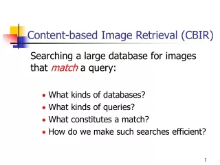
Image Retrieval by Content (CBIR)
1.47k likes | 2.65k Views
Image Retrieval by Content (CBIR). Presentation Outline. Introduction History of image retrieval – Issues faced Solution – Content-based image retrieval Feature extraction Multidimensional indexing Current Systems Open issues Conclusion. Introduction.

Image Retrieval by Content (CBIR)
E N D
Presentation Transcript
Presentation Outline • Introduction • History of image retrieval – Issues faced • Solution – Content-based image retrieval • Feature extraction • Multidimensional indexing • Current Systems • Open issues • Conclusion
Introduction • Image databases, once an expensive proposition, in terms of space, cost and time has now become a reality. • Image databases, store images of a various kinds. • These databases can be searched interactively, based on image content or by indexed keywords.
Introduction Examples: • Art collection – paintings could be searched by artists, genre, style, color etc. • Medical images – searched for anatomy, diseases. • Satellite images – for analysis/prediction. • General – you want to write an illustrated report.
Introduction Database Projects: • IBM Query by Image Content (QBIC). • Retrieves based on visual content, including properties such as color percentage, color layout and texture. • Fine Arts Museum of San Francisco uses QBIC. • Virage Inc. Search Engine. • Can search based on color, composition, texture and structure.
Introduction Commercial Systems: • Corbis – general purpose, 17 million images, searchable by keywords. • Getty Images – image database organized by categories and searchable through keywords. • The National Laboratory of Medicine – database of X-rays, CT-scans MRI images, available for medical research. • NASA & USGS – satellite images (for a fee!)
History of Image Retrieval • Images appearing on the WWW typically contain captions from which keywords can be extracted. • In relational databases, entries can be retrieved based on the values of their textual attributes. • Categories include objects, (names of) people, date of creation and source. • Indexed according to these attributes.
History of Image Retrieval • Traditional text-based image search engines • Manual annotation of images • Use text-based retrieval methods • E.g. Water lilies Flowers in a pond <Its biological name>
History of Image Retrieval SELECT * FROM IMAGEDB WHERE CATEGORY = ‘GEMS’ AND SOURCE = ‘SMITHSONIAN’
History of Image Retrieval SELECT * FROM IMAGEDB WHERE CATEGORY = ‘GEMS’ AND SOURCE = ‘SMITHSONIAN’ AND (KEYWORD = ‘AMETHYST’ OR KEYWORD = ‘CRYSTAL’ OR KEYWORD = ‘PURPLE’)
Limitations of text-based approach • Problem of image annotation • Large volumes of databases • Valid only for one language – with image retrieval this limitation should not exist • Problem of human perception • Subjectivity of human perception • Too much responsibility on the end-user • Problem of deeper (abstract) needs • Queries that cannot be described at all, but tap into the visual features of images.
Outline • History of image retrieval – Issues faced • Solution – Content-based image retrieval • Feature extraction • Multidimensional indexing • Current Systems • Open issues • Conclusion
What is CBIR? • Images have rich content. • This content can be extracted as various content features: • Mean color , Color Histogram etc… • Take the responsibility of forming the query away from the user. • Each image will now be described by its own features.
CBIR – A sample search query • User wants to search for, say, many rose images • He submits an existing rose picture as query. • He submits his own sketch of rose as query. • The system will extract image features for this query. • It will compare these features with that of other images in a database. • Relevant results will be displayed to the user.
Outline • History of image retrieval – Issues faced • Solution – Content-based image retrieval • Feature extraction • Multidimensional indexing • Current Systems • Open issues • Conclusion
Feature Extraction • What are image features? • Primitive features • Mean color (RGB) • Color Histogram • Semantic features • Color Layout, texture etc… • Domain specific features • Face recognition, fingerprint matching etc… General features
Mean Color • Pixel Color Information: R, G, B • Mean component (R,G or B)= Sum of that component for all pixels Number of pixels Pixel
Histogram • Frequency count of each individual color • Most commonly used color feature representation Corresponding histogram Image
Color Layout • Need for Color Layout • Global color features give too many false positives • How it works: • Divide whole image into sub-blocks • Extract features from each sub-block • Can we go one step further? • Divide into regions based on color feature concentration • This process is called segmentation.
Example: Color layout ** Image adapted from Smith and Chang : Single Color Extraction and Image Query
Color Similarity Measures • Color histogram matching could be used as described earlier. • QBIC defines its color histogram distance as ddist (I,Q) = (h(I) – h(Q))TA(h(I) – h(Q)) where h(I) and h(Q) are the K-bin histogram of images I and Q respectively and A is a KxK similarity matrix. • In this matrix similar colors have values close to1 and colors that are different have values close to 0.
Color Similarity Measures • Color layout is another possible distance measure. • The user can specify regions with specific colors. • Divide the image into a finite number of grids. Starting with an empty grid, associate each grid with a specific color (chosen from a color palette.
Color Similarity Measures • It is also possible to provide this information from a sample image. As was seen in Fig 8.3. • Color layout measures that use a grid require a grid square color distance measure dcolorthat compare the grids between the sample image and the matched image. • dgridded_square (I,Q) = Σ dcolor(CI(g),CQ(g)) g
Where CI(g) and CQ(g) represent the color in grid g of a database image I and query image Q respectively. • The representation of the color in a grid square can be simple or complicated. • Some suitable representations are • The mean color in the grid square • The mean and standard deviation of the color • A multi-bin histogram of the color • These should be assigned meaning ahead of time, i.e. mean color could mean representation of the mean of R, G and B or a single value.
Texture • Texture – innate property of all surfaces • Clouds, trees, bricks, hair etc… • Refers to visual patterns of homogeneity • Does not result from presence of single color • Most accepted classification of textures based on psychology studies – Tamura representation • Coarseness • Contrast • Directionality • Linelikeness • Regularity • Roughness
Segmentation issues • Considered as a difficult problem • Not reliable • Segments regions, but not objects • Different requirements from segmentation: • Shape extraction: High Accuracy required • Layout features: Coarse segmentation may be enough
Texture Similarity Measures • Texture similarity tends to be more complex use than color similarity. • An image that has similar texture to a query image should have the same spatial arrangements of color, but not necessarily that same colors. • The texture measurements studied in the previous chapter can be used for matching.
Texture Similarity Measures • In the previous example Laws texture energy measures were used. • As can be seen from the results, the measure is independent of color. • It also possible to develop measures that look at both texture and color. • Texture distance measures have two aspects • The representation of texture • The definition of similarity with respect to that representation
Texture Similarity Measures • The most commonly used texture representation is a texture description vector, which is a vector of numbers that summarizes the texture in a given image or image region. • The vector of Haralick’s five co-occurrence-based texture features and that of Laws’ nine texture energy features are examples.
Texture Similarity Measures • While a texture description vector can be used to summarize the texture in an entire image, this is only a good method for describing single texture images. • For more general images, texture description vectors are calculated at each pixel for a small (e.g. 15 x15) neighborhood about that pixel. • Then the pixels are grouped by a clustering algorithm that assigns a unique label to each different texture category it finds.
Texture Similarity Measures • Several distances can be defined once the vector information is derived for an image. The simplest texture distance is the pick-and-click approach, where the user picks the texture by clicking on the image. • The texture measure vector is found for the selected pixel and is used to measure similarity with the texture measure vectors for the images in the database.
Texture Similarity Measures • The texture distance is given by dpick_and_click(I,Q)= min i in I ||T(i) – T(Q)||2 where T(i) is the texture description vector at pixel I of the image I and T(Q) is the textue description vector at the selected pixel (or region). • While this could be computationally expensive to do on the fly, prior computation (and indexing) of the textures in the image database would be a solution.
Alternate to pick-and-click is the gridded approach discussed in the color matching. • A grid is placed on the image and texture description vector calculated for the query image. The same process is applied to the DB images. • The gridded texture distance is given by • Where dtexture can be Euclidean distance or some other distance metric.
Shape Similarity Measures • Color and texture are both global attributes of an image. • Shape refers to a specific region of an image. • Shape goes one step further than color and texture in that it requires some kind of region identification process to precede the shape similarity measure. • Segmentation is still a crucial problem to be solved. • Shape matching will be discussed here.
Shape Similarity Measures • 2-D shape recognition is an important aspect of image analysis. • Comparing shapes can be accomplished in several ways – structuring elements, region adjacency graphs etc. • They tend to expensive in terms of time. • In CBIR we need the shape matching to be fast. • The matching should also be size, rotational and translation invariant.
Shape Histogram • Histogram distance simply an extension from color and texture. • The biggest challenge is to define the variable on which the histogram is defined. • One kind of histogram matching is projection matching, using horizontal and vertical projections of the shape in a binary image.
Projection Matching • For an n x m image construct an n+m histogram where each bin will contain the number of 1-pixels in each row and column. • This approach is useful if the shape is always the same size. • To make PM size invariant, n and m are fixed • Translation invariance can be achieved in PM by shifting the histogram from the top-left to the bottom-right of the shape.
Projection Matching • Rotational invariance is harder but can be achieved by computing the axes of the best fitting ellipse and rotate the shape along the major axis. • Since we do not know the top of the shape we have to try two orientations. • If the major and minor-axes are about the same size four orientations are possible.
Projection Matching • Another possibility is to construct the histogram over the tangent angle at each pixel on the boundary of the shape. • This is automatically size and translation but not rotation invariant. • The rotational invariance can be solved by rotating the histogram (K possible rotations in a K-bin histogram).
Boundary Matching • BM algorithms require the extraction and representation of the boundaries of the query shape and image shape. • The boundary can be represented as a sequence of pixels or maybe approximated by a polygon. • For a sequence of pixels, one classical matching technique uses Fourier descriptors to compare two shapes.
Boundary Matching • In the continuous case the FDs are the coefficients of the Fourier series expansion of the function that defines the boundary of the shape. • In the discrete case the shape is represented by a sequence of m points <V0, V1, …,Vm-1>. • From this sequence of points a sequence of unit vectors and a sequence of cumulative differences can be computed
Boundary Matching • Unit vectors – • Cumulative differences
Boundary Matching • The Fourier descriptors {a-M, …, a0, …,aM} are then approximated by • These descriptors can be used to define a shape distance measure.
Boundary Matching • Suppose Q is the query shape and I is the image shape. Let {anQ} be the sequence of FDs for the query and {anI} be the sequence of FDs for the image. • The the Fourier distance measure is given by
Boundary Matching • This measure is only translation invariant. • Other methods can be used in conjunction with this to solve other invariances. • If the boundary is represented by polygons, the lengths and angles between them can be used to compute and represent the shapes.