System Modeling with Petri Nets
System Modeling with Petri Nets. Andrea Bobbio and Kishor Trivedi Dipartimento di Informatica Universit à del Piemonte Orientale, 15100 Alessandria (Italy) bobbio@unipmn.it - URL: www.mfn.unipmn.it/~bobbio Center for Advanced Computing and Communication (CACC)

System Modeling with Petri Nets
E N D
Presentation Transcript
System Modeling with Petri Nets Andrea Bobbio and Kishor Trivedi Dipartimento di Informatica Università del Piemonte Orientale, 15100 Alessandria (Italy) bobbio@unipmn.it - URL:www.mfn.unipmn.it/~bobbio Center for Advanced Computing and Communication (CACC) Department of Electrical and Computer Engineering Duke University, Durham, NC 27708-0291(USA) kst@ee.duke.edu - URL: www.ee.duke.edu/~kst Duke University, November 2003
Outline • What are Petri Nets; • Definitions and basic concepts; • Examples; • Stochastic Petri Net (SPN); • Generalized SPN and Stochastic Reward Net (SRN). A Monograph on this subject is: http://www.mfn.unipmn.it/~bobbio/BIBLIO/PAPERS/ANNO90/kluwerpetrinet.pdf
Petri Nets • Petri Nets (PN) are a graphical paradigm for the formal description of the logical interactions among parts or of the flow of activities in complex systems. • PN are particularly suited to model: • Concurrency and Conflict; • Sequencing, conditional branching and looping; • Synchronization; • Sharing of limited resources; • Mutual exclusion.
Petri Nets Petri Nets (PN) originated from the Phd thesis of Carl Adam Petri in 1962. A web service on PN is managed at the University of Aarhus in Denmark, where a bibliography with more that 8,500 items can be found. http://www.daimi.au.dk/PetriNets/ • Regular International Conferences: • ATPN - Application and Theory of PN • PNPM – PN and Performance Models
Petri Nets The original PN did not convey any notion of time. For performance and dependability analysis it is necessary to introduce the duration of the events associated to PN transitions. • Timed model were subsequently extensively explored, following two main lines: • Random durations : Stochastic PN (SPN) • Deterministic or interval: Timed PN (TPN)
Definitions • A Petri net (PN) is a bipartite directed graph consisting of two kinds of nodes: places and transitions • Places typically represent conditions within the system being modeled • Transitions represent events occurring in the system that may cause change in the condition of the system • Arcs connect places to transitions and transitions to places (never an arc from a place to a place or from a transition to a transition)
Example of a PN t1 p1 p2 t2 p1 – resource idle p2 – resource busy t1 – task arrives t2 – task completes
Example of a PN p3 t1 p1 p2 t2 p1 – resource idle p2 – resource busy p3 – user t1 – task arrives t2 – task completes
Definition of PN A PN is a n-tuple (P,T,I,O,M) P set of places T set of transitions I input arcs O output arcs M marking
PN Definitions • Input arcs are directed arcs drawn from places to transitions, representing the conditions that need to be satisfied for the event to be activated • Output arcs are directed arcs drawn from transitions to places, representing the conditions resulting from the occurrence of the event
PN Definitions • Input places of a transition are the set of places that are connected to the transition through input arcs • Output places of a transition are the set of places to which output arcs exist from the transition
PN Definitions • Tokens are dots (or integers) associated with places; a place containing tokens indicates that the corresponding condition holds • Marking of a Petri net is a vector listing the number of tokens in each place of the net m (m1m2 … mP) ; P = # of Places
PN Definitions • When input places of a transition have the required number of tokens, the transition is enabled. • An enabled transition may fire (event happens) removingone token from each input place and depositing one token in each of its output place.
Basic Components of PN input place transition output place token input arc output arc
The firing rules of a PN m t k m'
Enabling & Firing of Transitions up up up “t_fail” fires “t_fail” fires t_repair t_fail t_repair t_fail t_repair t_fail “t_repair” fires “t_repair” fires down down down A 2-processor failure/repair model
Reachability Analysis • A marking is reachable from another marking if there exists a sequence of transition firings starting from the original marking that results in the new marking • The reachability set of a PN is the set of all markings that are reachable from its initial marking
Reachability Analysis • A reachability graph is a directed graph whose nodes are the markings in the reachability set, with directed arcs between the markings representing the marking-to-marking transitions • The directed arcs are labeled with the corresponding transition whose firing results in a change of the marking from the original marking to the new marking
Generation of the reachability graph • By properly identifying the frontier nodes, the generation of the reachability graph involves a finite number of steps, even if the PN is unbounded. • Three type of frontier nodes: • terminal (dead) nodes: no transition is enabled; • duplicate nodes: already generated; • infinitely reproducible nodes.
Infinitely reproducible nodes A marking M´´ is an infinitely reproducible node if: M´´ M´ m i´´ m i´ (i= 1,2 …., nplace) where M´ is a marking already generated. In fact, the sequence M´ M´´ is firable from M´´ and then is infinitely reproducible. An arbitrarily large number of tokens is represented by a special symbol
Generation of an unbounded RG Producer/consumer
Extensions of PN models • arc multiplicity • inhibitor arcs • priority levels • enabling functions (guards) Note: The last three extensions destroy the infinitely reproducible property.
Petri Net: Arc Multiplicity • An arc cardinality (or multiplicity) may be associated with input and output arcs, whereby the enabling and firing rules are changed as follows: • Each input place must contain at least as many tokens as the cardinality of the corresponding input arc. • When the transition fires, it removes as many tokens from each input place as the cardinality of the corresponding input arc, and deposits as many tokens in each output places as the cardinality of the corresponding output arc. m p
Petri Net : Inhibitor Arc pi Inhibitor arcs are represented with a circle-headed arc. tk pj The transition can fire iff the inhibitor place does not contain tokens.
Petri Net : Multiple Inhibitor Arc • An inhibitor arc drawn from place to a transition means that the transition cannot fire if the corresponding inhibitor place contains at least as many tokens as the cardinality of the corresponding inhibitor arc • Inhibitor arcs are represented graphically as an arc ending in a small circle at the transition instead of an arrowhead n m p
An Example: Before or cardinality of the output arc
An Example: After or cardinality of the output arc
Priority levels A priority level can be attached to each PN transition. The standard execution rules are modified in the sense that, among all the transitions enabled in a given marking, only those with associated highest priority level are allowed to fire.
Enabling Functions An enabling function (or guard) is a boolean expression composed with the PN primitives (places, trans, tokens). The enabling rule is modified in the sense that beside the standard conditions, the enabling function must evaluate to true. pi tk (tk) = #P1<2 & #P2=0 pj
High Level (colored) Petri Nets In standard PN tokens are indistinguishable entities. The semantics of the model does not allow to follow the behavior of an individual token through the PN. High Level PN overcome this limitation by assigning to each individual token an attribute (color). Places, arcs and transitions can have functions and guards depending on the colors.
Colored Petri Nets t p <x> x C xC <x> C is a set of colors of cardinality |C| and x is an element of the set. Place p can contain tokens of any color x C; Transition t can fires tokens of any color x C.
Stochastic Petri Nets (SPN) • Petri nets are extended by associating time with the firing of transitions, resulting in timed Petri nets. • A special case of timed Petri nets is stochastic Petri net (SPN) where the firing times are considered random variables.
Stochastic Petri Nets (SPN) • A special case of stochastic Petri net (SPN) is where the firing times are exponentially distributed. • The marking process is mapped into a continuous time Markov chain (CTMC) with state space isomorphic to the reachability graph of the PN.
SPN: A Simple Example Server Failure/Repair t1 t1 . . p1 p2 p1 p2 t2 t2 Reachability graph CTMC t1 10 01 10 01 t2
SPN: Poisson Process PP with rate SPN model RG = CTMC 0 1 2 .......
SPN: M/M/1 Queue M/M/1 SPN model RG = CTMC 0 1 2 .......
SPN: M/M/1/n Queue (1) M/M/1/n n n SPN model RG = CTMC 0 1 2 ....... n
SPN: M/M/1/n Queue (2) M/M/1/n n SPN model n RG = CTMC 0 1 2 ....... n