Download
1 / 27
280 likes | 612 Views
Explore sinusoidal forcing, frequency response, amplitude ratios, phase shifts, Bode diagrams, time delays, and feedback controllers in system analysis. Learn shortcut techniques and plot interpretations for accurate frequency response identification.

E N D
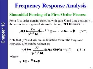
Sinusoidal Forcing of a First-Order Process • Frequency Response Analysis For a first-order transfer function with gain K and time constant , the response to a general sinusoidal input, is: Note that y(t) and x(t) are in deviation form. The long-time response, yl(t), can be written as: where:
Figure 13.1 Attenuation and time shift between input and output sine waves (K= 1). The phase angle of the output signal is given by , where is the (period) shift and P is the period of oscillation.
Frequency Response Characteristics of a First-Order Process • The output signal is a sinusoid that has the same frequency, w, as the input.signal, x(t) =Asinwt. • The amplitude of the output signal, , is a function of the frequency w and the input amplitude, A: 3. The output has a phase shift, φ, relative to the input. The amount of phase shift depends on w.
Dividing both sides of (13-2) by the input signal amplitude A yields the amplitude ratio (AR) which can, in turn, be divided by the process gain to yield the normalized amplitude ratio (ARN)
Shortcut Method for Finding the Frequency Response The shortcut method consists of the following steps: Step 1. Set s=jw in G(s) to obtain . Step 2. Rationalize G(jw); We want to express it in the form. G(jw)=R + jI where R and I are functions of w. Simplify G(jw) by multiplying the numerator and denominator by the complex conjugate of the denominator. Step 3. The amplitude ratio and phase angle of G(s) are given by: Memorize
Example 13.1 Find the frequency response of a first-order system, with Solution First, substitute in the transfer function Then multiply both numerator and denominator by the complex conjugate of the denominator, that is,
where: From Step 3 of the Shortcut Method, or Also,
Complex Transfer Functions Consider a complex transfer G(s), Substitute s=jw, From complex variable theory, we can express the magnitude and angle of as follows:
Bode Diagrams • A special graph, called the Bode diagram or Bode plot, provides a convenient display of the frequency response characteristics of a transfer function model. It consists of plots of AR and as a function of w. • Ordinarily, w is expressed in units of radians/time. Bode Plot of A First-order System Recall:
Note that the asymptotes intersect at , known as the break frequency or corner frequency. Here the value of ARN from (13-21) is: • Some books and software defined AR differently, in terms of decibels. The amplitude ratio in decibels ARd is defined as
Integrating Elements The transfer function for an integrating element was given in Chapter 5: Second-Order Process A general transfer function that describes any underdamped, critically damped, or overdamped second-order system is
Substituting and rearranging yields: Figure 13.3 Bode diagrams for second-order processes.
Time Delay Its frequency response characteristics can be obtained by substituting , which can be written in rational form by substitution of the Euler identity, From (13-54) or
Figure 13.7 Phase angle plots for and for the 1/1 and 2/2 Padé approximations (G1 is 1/1; G2 is 2/2).
Process Zeros Consider a process zero term, Substituting s=jw gives Thus: Note: In general, a multiplicative constant (e.g., K) changes the AR by a factor of K without affecting .
Frequency Response Characteristics of Feedback Controllers Proportional Controller. Consider a proportional controller with positive gain In this case , which is independent of w. Therefore, and
Proportional-Integral Controller. A proportional-integral (PI) controller has the transfer function (cf. Eq. 8-9), Substitute s=jw: Thus, the amplitude ratio and phase angle are:
Ideal Proportional-Derivative Controller. For the ideal proportional-derivative (PD) controller (cf. Eq. 8-11) The frequency response characteristics are similar to those of a LHP zero: Proportional-Derivative Controller with Filter. The PD controller is most often realized by the transfer function
Figure 13.10 Bode plots of an ideal PD controller and a PD controller with derivative filter. Idea: With Derivative Filter:
PID Controller Forms • Parallel PID Controller. The simplest form in Ch. 8 is Series PID Controller. The simplest version of the series PID controller is Series PID Controller with a Derivative Filter.
Figure 13.11 Bode plots of ideal parallel PID controller and series PID controller with derivative filter (α = 1). Idea parallel: Series with Derivative Filter:
Nyquist Diagrams Consider the transfer function with and
Figure 13.12 The Nyquist diagram for G(s) = 1/(2s + 1) plotting and
Figure 13.13 The Nyquist diagram for the transfer function in Example 13.5: