Frequency Response
EGR 272 – Frequency Response using MATLAB. Frequency Response The output of many circuits varies as frequency varies. This behavior can be beneficial as circuits can be designed to block or pass signals in certain frequency ranges. Consider the three cases shown below:.


Frequency Response
E N D
Presentation Transcript
EGR 272 – Frequency Response using MATLAB Frequency Response The output of many circuits varies as frequency varies. This behavior can be beneficial as circuits can be designed to block or pass signals in certain frequency ranges. Consider the three cases shown below: Low Pass Filter (LPF) Allows only low frequencies to pass and block high frequencies. Band Pass Filter (BPF) Allows only frequencies in a certain range to pass. Example: tuner on a radio which blocks all frequencies (radio stations) except the one that you select. High Pass Filter (HPF) Allows only high frequencies to pass and block low frequencies.
EGR 272 – Frequency Response using MATLAB Transfer Functions: Determining the frequency response begins with finding the transfer function, H(s). H(s) is defined as follows:
EGR 272 – Frequency Response using MATLAB • Graphing frequency response - Procedure: • Form H(jw) by replacing s with jw in H(s). • Since H(jw) is a complex function it can be expressed in polar form with a magnitude and an angle as follows: H(jw) = |H(jw)| (w) • Frequency response is generally illustrated by graphing one of the following: • Magnitude response: Graph of |H(jw)| vs w • Log-Magnitude (LM) response: Graph of 20 log |H(jw)| vs w • Phase response: Graph of (w) vs w • Note that |H(jw)| is typically a unitless quantity (|Vo/Vin| or |Io/Iin| for example), but • 20 log |H(jw)| has the units of decibels, dB.
EGR 272 – Frequency Response using MATLAB Example: For the transfer function above, find H(jw) and graph the LM response and the phase response using MATLAB. Let w vary from 1 to 1000 rad/s. Note: This is the exact function used to form the LM response for the LPF on the first slide. Recall that in MATLAB we can use the functions: abs( )- finds the magnitude of a complex number (or transfer function) angle( )– finds the phase of a complex number (or a transfer function)
EGR 272 – Frequency Response using MATLAB Class Example: Use MATLAB to graph the LM and phase response for the transfer function below. Use a technique similar to the last example using the abs( )and angle( ) functions. Note: This is the exact function used to form the LM response for the BPF on the first slide.
EGR 272 – Frequency Response using MATLAB • Functions in MATLAB for frequency response • Frequency response is such an important topic in EE that some special functions are available in MATLAB to make finding frequency response easier. In EGR 272 we introduce Bode plots as good approximations for frequency response. We often find: • Bode LM plot • Bode phase plot • Oddly, the function bode( ) in MATLAB can be used to find exact frequency response plots (not approximations). Consider the functions described on the following slide:
EGR 272 – Frequency Response using MATLAB MATLAB functions useful for finding frequency response tf(N,D) – finds a transfer function given a numerator, N, and a denominator, D, (expressed as polynomials) Example: N = [1 20]; // represents the numerator (s + 20) D = [1 100]; // represents the denominator (s + 100) H = tf(N,D); // forms (and displays) the transfer function H = (s + 20)/(s + 100) bode(H)– creates LM and phase plots for transfer function H over a range of frequency selected by MATLAB bode(H,w)– similar to bode(H), but uses the range of frequency, w, specified by the user. For example, the user might specify: w = logspace(2,4,50); bode(H,{w1,w2})– similar to bode(H), but uses the frequency range from w1 to w2. freqresp( )– can be used to generate a vector a points for frequency response, but we won’t use it here as bode( )is more convenient.
EGR 272 – Frequency Response using MATLAB Example: Repeat the earlier example of graphing the LM and phase responses for H(s), but use the tf( )and bode( )functions. Output from tf( ) command
EGR 272 – Frequency Response using MATLAB Class Example: Use MATLAB to graph the LM and phase response for the transfer function below using the tf( )and bode( )functions. Note that the results should match an earlier example.