Frequency Response: Nyquist Analysis & Design
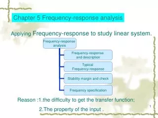
Frequency Response: Nyquist Analysis & Design. Or Elements of Complex Variables. Mathematical Foundation: Fundamental Theory of Linear Systems. The steady state response of a stable linear time invariant system to a sinusoidal input with frequency w input is


Frequency Response: Nyquist Analysis & Design
E N D
Presentation Transcript
Frequency Response: Nyquist Analysis & Design Or Elements of Complex Variables
Mathematical Foundation: Fundamental Theory of Linear Systems • The steady state response of a stable linear time invariant system to a sinusoidal input with frequency winput is • A sinusoid at the same frequency of the input • Whose magnitude is the magnitude of the input multiplied by the magnitude of the transfer function evaluated at s=jwinput • Whose phase is the sum of the phase of the input and the angle of the transfer function evaluated at s=jwinput
Translate into mathematics Input Transfer function SS output
Implications of FTLS • Transfer functions tell us what to expect from experimental frequency response data (see exercise 1) • Experimental Frequency response data tells us about transfer functions (see exercise 2) • Bode design techniques • Open loop transfer functions tell us about stability of closed loop systems (Basic idea to be explored)
Ex 1. TF to expected frequency response data • Generate raw experimental data. Choose a transfer function H(s). Use Sysquake (or MatLab, or MathCAD, or …) to find its complete response to sinusoids with amplitude A (you choose) and at 5 widely spaced frequencies (you choose). • Analyze your raw data. Based on the plots obtained in step 1, find the amplitude and phase of the steady-state response • Theoretical prediction. Use the FTLS, the H(s), frequencies, and amplitude from step 1 to predict the steady state amplitudes and phases. • Comparison. Compare the theoretical predictions to the results of you analysis of raw data. • Conclusion. Is the FTLS valid? Why is it important that you choose the TF and the frequencies rather than me?
Ex 2a. FR data to TF: 1st order system • Given experimentally determined FR data (possibly corrupted by measurement noise) determine the best 1st order TF that summarizes the data. (Theory as data compactor) • Number of TF parameters • Minimum number of required data points • Dealing with noise
Ex 2b. FR data to TF: 2nd order system • Given experimentally determined FR data (possibly corrupted by measurement noise) determine the best 2nd order TF that summarizes the data. (Theory as data compactor) • Number of TF parameters • Minimum number of required data points • Dealing with noise
2 0 -2 0 10 20 Ex 2b Data: A=2, w=2
5 0 -5 0 20 40 Ex 2b Data: A=2, w=1
5 0 -5 0 20 40 Ex 2b Data: A=2, w=5
2 0 -2 0 10 20 Ex 2b Data: A=?, w=?
2 0 -2 0 10 20 Ex 2b Data: A=?, w=?
2 0 -2 0 10 20 Ex 2b Data: A=?, w=?
function (t,y)=main() a=?; b=??; // unknown parameters A=2; w=2; // input data p=[a b A w]; T=max([1/b 2*pi/w]) timeinterval=[0,5*T]; IC=0; (t,y)=ode45(@f,timeinterval,IC,[],p); clf noise = (rand(1,length(y))-.5)'*max(y)/5; y=y+noise; plot(t',y','r') plot(t',A*cos(w*t)') timeinterval p return Sysquake Code to generate data // Generate frequency response data // (C) 2004 PD Olivier // H(s)=a/(s+b) function yp=f(t,y,p) //TF H(s)=a/(s+b) a=p(1); b=p(2); A=p(3); w=p(4); yp = -a*y+b*A*cos(w*t); return