Ernst Mayr
Ernst Mayr. “It is altogether unlikely that two genes would have identical selective values under all the conditions in which they exit… cases of neutral polymorphism do not exist… it appears probable that random fixation is of negligible evolutionary importance’. Lewontin and Hubby, 1966.

Ernst Mayr
E N D
Presentation Transcript
Ernst Mayr “It is altogether unlikely that two genes would have identical selective values under all the conditions in which they exit… cases of neutral polymorphism do not exist… it appears probable that random fixation is of negligible evolutionary importance’
Lewontin and Hubby, 1966 • Calculated the proportion of polymorphic loci in Drosophila. • Argued that NS could not actively maintain so much genetic variation, and suggested that much of it might be selectively neutral.
Neutral Theory of Molecular Evolution • Kimura, 1968 Holds that although a small minority of mutations in DNA or protein sequences are adv., and are fixed by NS, and although some are disadv. and are eliminated by ‘purifying’ NS, the great majority of mutations that are fixed are effectively neutral with respect to fitness, and are fixed by genetic drift.
THUS, Most genetic variation at the molecular level is selectively neutral and lacks adaptive significance Does not hold that the morphological, physiological and behavioral features of organisms evolve by RGD, such features evolve chiefly by NS
Selection does occur in NT • Most variation has little effect on fitness
Testing the Neutral theory • Synonymous vs Nonsynonymous substitutions • Microadaptation within protein coding genes • Types of selection “positive”
Evolutionary change in Nucleotide sequence • Basic Process • Estimating rates of substitution • Reconstructing organism phylogeny
Compare two or more sequences descended from a common ancestor
Purines Pyrimidines A G C T
Models of Nucleotide Sub. • Jukes-Cantor • assumes that all nucleotides are present with equal frequencies • assumes equal probabilities for all possible nucleotide substitutions • Kimura 2-parameter • assumes that all nucleotides are present with equal frequencies • assumes Ti () and Tv (β) probabilities are different
3 Sub. Types Tv, 2 Ti Equal base frequencies 3 Sub. Types 2 Tv classes, Ti 2 Sub. Types Tv vs. Ti Equal base frequencies 2 Sub. Types Tv vs. Ti Single sub. type Equal base frequencies Single sub. type GTR TrN SYM K3ST HKY85 F84 F81 K2P JC
Jukes and Cantor (1969) • If you have an A at site i it will change to G, T, C with equal probability • Thus the rate of substitution per unit time is 3. • The rate of sub. in each of the 3 possible directions of change is
Jukes and Cantor (1969) cont. • What is the prob. that this site is occupied by A at time t? PA(t) • The prob. that this site is occupied by A at time 0 isPA(0)=1and still having A time 1 PA(1)= 1-3
Jukes and Cantor (1969) cont. A A T=0 No sub. sub. Not A A T=1 No sub. sub. A A T=2 The prob. of A at time 2 is PA(2) = (1-3) PA(1)+[1-PA(1)]
Purines Pyrimidines Kimura 2 Parameter A G β β C T
Kimura Scenario’s A A A A T=0 No sub. Ti. Tv. Tv. T=1 G A C T No sub. Ti. Tv. Tv. T=2 A A A A
3 Sub. Types Tv, 2 Ti Equal base frequencies 3 Sub. Types 2 Tv classes, Ti 2 Sub. Types Tv vs. Ti Equal base frequencies 2 Sub. Types Tv vs. Ti Single sub. type Equal base frequencies Single sub. type GTR TrN SYM K3ST HKY85 F84 F81 K2P JC
Substitutions Time 0 Outgroup) ATGTCAGGGACTCAGATCGAATGGGATCTAG Taxon 1) .....C......T.................. Taxon 2) .....G......T........C......... Taxon 3) .....C...........A............. Taxon 4) .....G...........A........G....
Substitutions Time 1 Outgroup) ATGTCAGGGACTCAGATCGAATGGGATCTAG Taxon 1) .....A......T.................. Taxon 2) .....G......G........C......... Taxon 3) .....G...........A............. Taxon 4) .....G...........A........G....
Substitutions Time 2 Outgroup) ATGTCAGGGACTCAGATCGAATGGGATCTAG Taxon 1) .....G......T.................. Taxon 2) .....G......T........C......... Taxon 3) .....G...........A............. Taxon 4) .....G...........A........G.... Multiple Substitutions at the same site
Hamming Distance or P=n/N*100 Outgroup) ATGTCAGGGACTCAGATCGAATGGGATCTAG Taxon 1) .....C......T.................. Taxon 2) .....G......T........C......... Taxon 3) .....C...........A............. Taxon 4) .....G...........A........G.... N=31 P=2/31*100=6.45%
Substitutions Time 2 Outgroup) ATGTCAGGGACTCAGATCGAATGGGATCTAG Taxon 1) .....G......T.................. Taxon 2) .....G......T........C......... Taxon 3) .....G...........A............. Taxon 4) .....G...........A........G.... A→C→G P=2/31*100=6.45%
Nucleotide diff. between seq. Prob. at time t = PAA(t) For both seq. the prob. at time t = P2AA(t)
I(t) = Prob. That the nucleotide at a given site at time t is the same in both sequences I(t) = P2AA(t) + P2 AT(t) P2AC(t) + P2AG(t)
Same as in the JC For 2 sequences Note that the prob. the 2 seq. are different at the site at time t is P = 1-I(t)
JC model Problem, we do not know t
K = the # of substitutions per site since the time of divergence between the two sequences K = 2(3t) where (3t) is the number of sub. between a single lineage
JC model # of substitutions per site since the time of divergence
Table 3.2 The one-parameter (jukes and Cantor 1969) and four-parameter (Blaisdell 1985) schemes of nucleotide substitution in matrix forma
3 Sub. Types Tv, 2 Ti Equal base frequencies 3 Sub. Types 2 Tv classes, Ti 2 Sub. Types Tv vs. Ti Equal base frequencies 2 Sub. Types Tv vs. Ti Single sub. type Equal base frequencies Single sub. type GTR TrN SYM K3ST HKY85 F84 F81 K2P JC
So Which model? • Multiple assumptions (= nuc. freq. to start etc). • Sampling errors due to the use of logarithmic functions (zero).
Protein encoding genes • Synonymous and Nonsynonymous • Very difficult as a site changes over time • CGG (arg) 3rd postion is syn. But if 1st pos mutates to T then the 3rd position of the resulting codon becoming Nonsynonymous • Many sites are not completely synonymous or nonsynonymous • Depending the type of mutation, a TI at the 3rd position of CGG (arg) is syn, whereas a TV is nonsynonymous
Multiple ways to calculate Ks & Ka • Li et al., 1985 • Classify the nucleotides into: • nondegenerate: all changes at the site are nonsyn. • twofold degenerate: 1 of 3 is synonymous • fourfold degenerate: all 3 are syn.
Categorize degeneracy, • Further separate on mutation types (transitional, or transversional) for each type of degeneracy. • Ks: the number of synonymous substitutions per synonymous site • Ka: the number of nonsynonymous substitutions per nonsynonymous site
Why? • Study evolution • Positive selection • Negative selection