Hydrologic connectivity from hillslope to landscape scales:

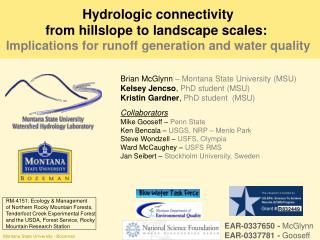
1. Hydrologic connectivity from hillslope to landscape scales: Implications for runoff generation and water quality R832449 Brian McGlynn – Montana State University (MSU) Kelsey Jencso, PhD student (MSU) Kristin Gardner, PhD student (MSU) Collaborators Mike Gooseff – Penn State Ken Bencala –USGS, NRP – Menlo Park Steve Wondzell –USFS, Olympia Ward McCaughey –USFS RMS Jan Seibert – Stockholm University, Sweden RM-4151: Ecology & Managementof Northern Rocky Mountain Forests, Tenderfoot Creek Experimental Forest and the USDA, Forest Service, Rocky Mountain Research Station EAR-0337650 - McGlynn EAR-0337781 - Gooseff

2. Does spatial location of change influence watershed response to perturbation?Big Sky, Montana an outdoor laboratory Residences (septic systems) increasing by 100s per year • Requires: • understanding of hydrologic connectivity across landscape • relationships between pattern of change and landscape structure

3. OBJECTIVES Investigate hydrologic connectivity over space and time Develop conceptual model of runoff generation–watershed structure Test ideas in a developing watershed (Big Sky) – applied example Tenderfoot Creek Experimental Forest Map area ~ 22 km2 7 gauged watersheds

4. Hydrologic instrumentation 24 transects of nested wells and piezometers (140 recording GW wells) 7 flumes with real time specific conductance (SC), temperature, and stage recorders ALSM 1m topography data 9 water content probe nests across riparian hillslope transitions >8 rain gauges 4 snowmelt lysimeters 2 SNOTEL sites 2 H2O/CO2 eddy-covariance towers w/ full energy budget instrumentation. 600 m2 plot w/ intense water content (64 TDR probes) soil and snow temperature (80) Frequent stream and GW sampling with a focus on solutes, 18O, D, and DOC Tenderfoot Creek Experimental Forest (USFS) (USFS) Stringer Creek Stringer Creek Spring Park Spring Park Creek Creek ~22 km2 Lower Lower Tenderfoot Tenderfoot Creek Creek Upper Tenderfoot Creek Upper Tenderfoot Creek Bubbling Bubbling Sun Creek Sun Creek Creek Creek 0 0 250 250 500 500 1,000 1,000 Meters Meters Snow Snow Lysimeter Lysimeter Eddy Flux Tower Eddy Flux Tower Snow Lysimeter SNOTEL SNOTEL Flume Flume Well Transect Well Transect Little Belt Mountains, Montana ~850 mm precipitation with ~550 mm ET ~75% as snow 0 degrees C average temperature Soil depths 1-2 meters Elevation range ~500m from 2300m base Highly instrumented USFS nested catchments with a focus on water and carbon research from the plot to multiple watershed scales

5. Topographically-driven redistribution of water 0 ha Log10 40 ha Terrain-based riparian mapping

6. Combining upland drainage and local riparian area along the stream network Buffering potential f (riparian area : hillslope area) Low riparian buffer potential High riparian buffer potential Low to High riparian buffer potential > area accumulation > water accumulation > increase in streamflow Upland area accumulation pattern 0 ha Area accumulation 40 ha Hillslope area accumulation Hilllsope area accumulation stream

7. Lateral inflows vary along the channel network Riparian buffering potential varies along the channel network Riparian buffering potential frequency Buffering potential

8. Hillslope-riparian-stream hydrologic connectivity North hillslope North riparian Connectivity South hillslope South riparian 10/6 4/07 10/7 Water table elevation m NO CONNECTIVITY Kelsey Jencso

9. R2=0.91 n=24 Date

10. Examining watersheds in 4th dimension (temporal connectivity) Each side of the stream separated Max bar height = 100% Of the year

11. How does upland connectivity relate to streamflow magnitude?

12. Obj. 1: Investigate hydrologic connectivity over space and timeObj 2: Develop conceptual model of runoff generation–watershed structure Intermediate summary • Topographically driven lateral redistribution of water drives transient upland-stream connectivity and runoff generation • Riparian buffering potential spatially variable

13. Principles to apply to analysis of landuse change in the Big Sky watershed Hydrologic connectivity Riparian buffering potential Suggests location of change in watershed could be significant

14. Does spatial location of change influence watershed response to perturbation?Big Sky, Montana - an outdoor laboratory Resort • Residences (septic systems) increasing by 100s per year • Sampling locations

15. Weekly nitrate time series from 4 of 9 watersheds

16. Winter nitrate Maximum Value 2.17 mg/l Yellowstone Club – no access - Runoff mm/hr Nitrate mg/l

17. Late summer nitrate Maximum Value 1.31 mg/l Runoff mm/hr Nitrate mg/l

18. Stream nitrogen sources Human-derived nitrogen can be tracked with stable isotope analysis Natural range Septic impacted Atmospheric Deposition Geologic sources Septic 15N of dissolved N Stream samples across Big Sky watershed

19. Spatial structure of stream NSynoptic sampling variograms Distinct Seasonality in Spatial Dependence Flow connected Not flow connected No spatial correlation February October March SUGGESTS N immobilization in the growing season, leads to complex spatial patterns and a lack of spatial correlation June August September

20. Spatial Linear ModelsGeneralized Least Squares Estimation: Potential explanatory variables for stream nitrogen • # septics in subwatershed • # septics weighted by connectivity potential • geology (% shales) • stream order • % forest • riparian buffer potential (riparian area/hillslope area) • elevation • slope • roads • bare rock and talus • aspect • watershed area • and more… Methods: Cressie et al., 2006; Ver Hoef et al., 2006; Peterson et al., 2007.

21. Seasonal Influences on Streamwater Nitrate Dormant Season Growing Season Septic connectivity Riparian buffer pot. Geology N processing potential # Septics Geology N loading R2 = 0.9 R2 = 0.45 -0.53

22. Spatial Data Analysis Conclusions • Seasonality in variograms suggest N immobilization in uplands, riparian areas and stream network break down spatial patterns during growing season. • Spatial linear models indicate seasonality in the influences on streamwater NO3- • N loading variables significant during dormant season • Hydrologic connectivity and riparian buffer potential are significant during growing season Winter Summer

23. Take home message R832449 • Transient connectivity drives runoff generation (source areas change through time) • Watershed structure strong control on runoff generation and riparian buffering potential • Spatial location of change matters and intersection of change pattern and watershed hydrology influences response to perturbation *Gardner, K.K. and B.L. McGlynn. In revision. Spatio-Temporal Controls of Stream Water Nitrogen Export in a Rapidly Developing Watershed in the Northern Rockies. Water Resources Research. *Jencso, K. J., B. L. McGlynn, M. N. Gooseff, S. M. Wondzell, and K. E. Bencala. In revision. Hydrologic Connectivity Between Landscapes and Streams: Transferring Reach and Plot Scale Understanding to the Catchment Scale, Water Resources Research. EAR-0337650 - McGlynn EAR-0337781 - Gooseff

24. Extra slides to follow in case there are specific questions

25. Spatial Linear Models A B C [Cressie et al., 2006; Ver Hoef et al., 2006; Peterson et al., 2007. 1) Flow Connected vs Flow Unconnected 9 10 • Site B and C are flow-connected • Site A and C are flow-connected • Site A and B are not flow connected 10 2) Downstream Flow Distance (DFD) • BC = 20 • AC = 18 • AB = 19

26. Spatial Linear Models A B C 3) Proportional Influence of upstream site on downstream site FROM SITE TO SITE

27. Spatial Linear Models Generalized Least Squares Estimation: Covariance matrix (S)is a function of downstream distance (DFD),flow connectedness, and proportional influence. b= parameter estimates X = known explanatory variables z = known dependant variable (NO3-)