Download
1 / 66
820 likes | 1.4k Views
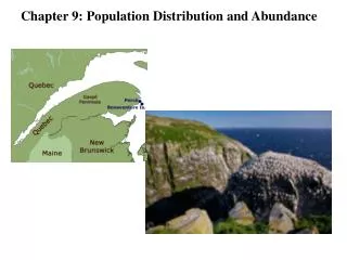
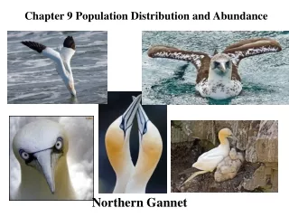
POPULATION DISTRIBUTION AND ABUNDANCE. Chapter 9. Chapter Concepts. Physical environment limits geographic distribution of species On small scales, individuals within pops. are distributed in random, regular, or clumped patterns; on larger scales, individuals within pop. are clumped

E N D
POPULATION DISTRIBUTION AND ABUNDANCE Chapter 9 Molles: Ecology 2nd Ed.
Chapter Concepts • Physical environment limits geographic distribution of species • On small scales, individuals within pops. are distributed in random, regular, or clumped patterns; on larger scales, individuals within pop. are clumped • Population density declines with increasing organism size • Rarity influenced by geographic range, habitat tolerance, pop. size; rare species vulnerable to extinction Molles: Ecology 2nd Ed.
Populations • Ecologists define a population as group of individuals of single species inhabiting specific area. Molles: Ecology 2nd Ed.
Habitat • Physical environmental conditions that allow individuals of species to survive AND reproduce Molles: Ecology 2nd Ed.
Habitat quality • Ability of environmental conditions to support repro and survival • Habitat area/volume • Resource concentration • Time • High habitat quality = organisms acquire many resources; high survival + repro = large pop. Molles: Ecology 2nd Ed.
Population numbers vary with habitat quality Molles: Ecology 2nd Ed.
Distribution Limits • Physical environment limits geographic distribution of species • Organisms can only compensate so much for environmental variation Molles: Ecology 2nd Ed.
Geographical range • Geographic area where species is found (based on macroclimate, salinity, nutrients, oxygen, light, etc.) Molles: Ecology 2nd Ed.
“Large-scale” patterns of distribution: • Refer to variation in species abundance w/in range • due to variation in habitat quality Molles: Ecology 2nd Ed.
Kangaroo Distributions and Climate • Caughley - relationship between climate + distribution of three largest kangaroos in Australia Molles: Ecology 2nd Ed.
Macropus giganteus – eastern greyEastern 1/3 of continenttemperate forest, tropical forest Molles: Ecology 2nd Ed.
Macropus fuliginosus – western grey southern and western regionstemperate woodlands and shrubs Molles: Ecology 2nd Ed.
Macropus rufus – redarid / semiarid interior Molles: Ecology 2nd Ed.
Fig 9.2 Distributions largely based on climate Molles: Ecology 2nd Ed.
Kangaroo Distributions and Climate • Limited distributions may not be directly determined by climate. • Climate often influences species distributions via: • food production • water supply • habitat • incidence of parasites, pathogens and competitors Molles: Ecology 2nd Ed.
Tiger Beetle of Cold Climates • Tiger beetle (Cicindela longilabris) - higher latitudes + elevations than other NA species • Schultz found metabolic rates of C. longilabris are higher and preferred temps. lower than other species • Physical env. limits species distributions Molles: Ecology 2nd Ed.
Fig 9.3 Metabolic rates of C. longilabris higher; preferred temps lower than other beetle species Adapted to cool climates Molles: Ecology 2nd Ed.
Distributions of Plants Along a Moisture-Temperature Gradient • Encelia spp. distributions + variations in temp and precipitation Fig 9.7 Molles: Ecology 2nd Ed.
Fig 9.5 Molles: Ecology 2nd Ed.
Distributions of Barnacles - Intertidal Gradient • Organisms in intertidal zone have evolved different degrees of resistance to drying • Barnacles - distinctive patterns of zonation within intertidal zone Molles: Ecology 2nd Ed.
Connell found pattern in barnacles: • Chthamalus stellatus restricted to upper levels; Balanus balanoides limited to middle and lower levels Molles: Ecology 2nd Ed.
Distributions of Barnacles Along an Intertidal Gradient • Balanus - more vulnerable to desiccation, excluded from upper intertidal zone • Chthamalus adults excluded from lower areas by competition with Balanus Molles: Ecology 2nd Ed.
Competition? How do we know that Balanus outcompetes Chthamalus? Molles: Ecology 2nd Ed.
Fig 9.8 Fig 9.9 Molles: Ecology 2nd Ed.
Distribution of Individuals on Small Scales • Three basic patterns: • Random: equal chance of being anywhere • Regular: uniformly spaced • Exclusive use of areas • Individuals avoid one another • Clumped: unequal chance of being anywhere • Mutual attraction between individuals • Patchy resource distribution Molles: Ecology 2nd Ed.
Fig 9.10 Molles: Ecology 2nd Ed.
Importance of scale in determining distribution patterns: • At one scale pattern may be random, at another scale, might be uniform: Molles: Ecology 2nd Ed.
Distribution of Tropical Bee Colonies • Hubbell and Johnson predicted aggressive bee colonies have regular distributions; • Predicted non-aggressive species have random or clumped distributions Molles: Ecology 2nd Ed.
Hubbell and Johnson results: • 4 species with regular distributions were highly aggressive • Fifth non-aggressive and randomly distributed Molles: Ecology 2nd Ed.
Fig 9.11 Molles: Ecology 2nd Ed.
What causes overall pattern? • Behavior! • Aggressive bees were uniformly spaced due largely to their interactions. • Non-aggressive species were random - did not interact. Molles: Ecology 2nd Ed.
Fig 9.10 Molles: Ecology 2nd Ed.
Distributions of Desert Shrubs • Traditional theory suggests desert shrubs are regularly spaced due to competition • Phillips and MacMahon - distribution of desert shrubs changes from clumped to regular patterns as they grow Molles: Ecology 2nd Ed.
Hypothesis: • Young shrubs clumped for (3) reasons: • Seeds germinate at safe sites • Seeds not dispersed from parent areas • Asexual reproduction Molles: Ecology 2nd Ed.
Distributions of Desert Shrubs • Phillips and MacMahon proposed as plants grow, some individuals in clumps die = reducing clumping • Competition among remaining plants produces higher mortality • Eventually creates regular distributions Molles: Ecology 2nd Ed.
Fig 9.13 - their hypothesis Molles: Ecology 2nd Ed.
Brisson and Reynolds • Dug up roots, map distribution of 32 bushes • found competitive interactions with neighboring shrubs influences distribution of creosote roots Molles: Ecology 2nd Ed.
So what? • Creosote bush roots do not overlap with nearby plant roots • Only 4% overlap between bushes Fig 9.14 Molles: Ecology 2nd Ed.
Distributions of Individuals on Large Scales • Bird Pops North America • Root - at continental scale, bird pops have clumped distributions (Christmas Bird Counts) • Clumped patterns in species with widespread distributions Molles: Ecology 2nd Ed. Fig 9.14
Similar distribution pattern for species with small range: few “hot spots”Fish crow Fig 9.14 Molles: Ecology 2nd Ed.
Brown et al. (1995) • Relatively few study sites gave most records for each bird species in Breeding Bird Survey (June): • clumped only during breeding season? Fig 9.16 Molles: Ecology 2nd Ed.
Density = number individuals per unit area/volume • Sedentary organisms: plot approach • Moving/secretive organisms: mark/recapture • Relative abundance = percent cover, CPUE Molles: Ecology 2nd Ed.
Estimating density • Sedentary animals and plants • Plot methods • Area of known size • Randomly located plots • Count individuals in plots • Average / plot • Density = average no. / plot area Molles: Ecology 2nd Ed.
(m + 1) Estimating density • Mobile or secretive animals: mark/recapture • 1. Sample animals and mark • 2. Release (M out of N in pop marked) • 3. Wait for mixing • 4. Sample (n), count how many marked (m) • 5. Compute estimate of pop size: • N = M (n + 1) Molles: Ecology 2nd Ed.
Example: Estimating Population Size from Mark-Recapture • Number of animals marked in 1st sample = 100 • Total number of animals in 2nd sample = 150 • Number of marked animals in 2nd sample = 11 Population = M (n + 1) = 100 (151) = 1258 Size (N) (m + 1) 12 Molles: Ecology 2nd Ed.
Another Example • Sample M = 38 squirrels, marked, released • After 2 weeks, resample, n = 120 • m = 12 of 120 marked • Estimate of pop. size: • N = M (n + 1) / (m + 1) • = 38 (120 + 1) / (12 + 1) = 353.7 • ~ 354 Molles: Ecology 2nd Ed.
Example: maple trees • 20 randomly located plots, 10 x 10 m squares (area = 100 m2) • Average sugar maple stems per plot = 4.5 • Unit area for trees = hectare (10,000 m2) • Density = 4.5 maples per plot / 0.01 hectare plots = 450 maples / ha Molles: Ecology 2nd Ed.
Example: zooplankters • 35 lake water samples, 50 ml each • Average copepods per sample = 78 • Unit volume for zooplankton = liters • Sample volume = 0.05 l • Density = 78 copepods per sample / 0.05 l samples • = 1560 copepods / l Molles: Ecology 2nd Ed.
Organism Size and Population Density • Population density decreases with larger organism size • Why? • Bigger organisms need more space and resources • Bigger organisms have lower repro rates Molles: Ecology 2nd Ed.
Damuth (1981) • Pop density of 307 spp. of herbivorous mammals decreased with increased body size Fig 9.19 Molles: Ecology 2nd Ed.